Localization Background

Bayes Filter

Monte Carlo Localization is a type of Bayes filter. You’ll remember the general Bayes Filter algorithm from the UKF project earlier in the course. This material is also covered in the EdX lectures for the class, which also contains mathematical derivations for the filter.

The Bayes Filter incorporates information available to the robot at each point in time to produce an accurate estimate of the robot’s position. Its core idea is to take advantage of data from two sources: the controls given to the robot and the measurements detected by the robot’s sensors.

At each new time step, the Bayes filter recursively produces a state estimate, represented as a probability density function called the belief. The belief assigns to every possible pose in the state space of the robot the probability that it is the robot’s true location. This probability is found in two steps called prediction and update.

The prediction step incorporates controls given to the robot between the previous state and the current one. It finds the probability of reaching a new state given the previous state and the control (hence recursion). The model used to find this probability is known as a state transition model and is specific to the robot in question.

The state transition model:
\(p(x_{t}|u_{t},x_{t-1})\)
ie. the probability that the most recent control \(u_t\) will transition the previous state \(x_{t-1}\) to the current state \(x_t\)

It is possible to estimate the state of the robot using only the prediction step and not incorporating the measurements taken by the robot’s sensors. This is known as dead reckoning. The dead reckoning estimate may be made more accurate by incorporating measurements from the robot’s sensors.

The Bayes filter does this in the update step by finding the probability that the current measurements are observed in the current state. The model used for this is known as a measurement model and is specific to the robot in question.

The measurement model:
\(p(z_{t}|x_{t})\)
ie. the probability that the current measurement \(z_t\) is observed given the state \(x_t\)

You may have noticed that each of the above steps required computing a probability stated like “the probability of x given y.” Such a probability is denoted \(p(X|Y)\) and may be calculated by the famous Bayes Theorem for conditional probabilities, hence the name of the algorithm.

Now, let’s take a look at the Bayes Filter:

\(\hspace{5mm} \text{Bayes\_Filter}(bel(x_{t-1}), u_{t}, z_{t}):\)
\(\hspace{10mm} \text{for all } x_t \text{ do}:\)
\(\hspace{15mm} \bar{bel}(x_t) = \int p(x_{t}|u_{t},x_{t-1})bel(x_{t-1})\mathrm{d}x\)
\(\hspace{15mm} bel(x_t) = \eta p(z_{t}|x_{t})\bar{bel}(x_t)\)
\(\hspace{10mm} \text{endfor}\)
\(\hspace{10mm} \text{return } bel(x_{t})\)

ie compute a belief by finding the probability of each possible new state. For each state, incorporate both the probability that the control transitions the previous state to this one and that the current measurements are observed in this state.

The first step \(\bar{bel}(x_t) = \int p(x_{t}|u_{t},x_{t-1})bel(x_{t-1})\mathrm{d}x\) is the motion prediction. \(\bar{bel}(x_t)\) represents the belief before the measurement is incorporated. The integral is computed discretely and becomes: \(\sum_x{p(x_t|u_t,x_{t-1})bel(x_{t-1})}\)

The second step \(bel(x_t) = \eta p(z_{t}|x_{t})\bar{bel}(x_t)\) is the measurement update. This computation is straightforward, the normalizer \(\eta\) is the reciprocal of the sum of \(p(z_{t}|x_{t})\bar{bel}(x_t)\) over all \(x_t\). This factor will normalize the sum.

Monte-Carlo Localization

The phrase “Monte Carlo” refers to the principle of using random sampling to model a complicated deterministic process. Rather than represent the belief as a probability distribution over the entire state space, MC localization randomly samples from the belief to save computational time. Because it represents the belief as samples, it is capable of representing multimodal distributions. For example when localizing, if the robot is teleported (i.e., turned off, and moved, and then turned on), its initial believe is uniform over the entire map. The Gaussian distribution has a hard time representing this, because its weight is centered on the mean (although you could approximate it with a very very large covariance). Another example is if the robot is experiencing aliasing. For example, if it is going down a long corridor, its observations at different points down the corridor will be exactly the same, until it reaches a distinguishing point, such as an intersection or the end of the corridor. Particle filters can represent this by having particles all along the corridor; whereas a Gaussian distribution will struggle because of the need to pick one place to center the distribution with the mean.

MC localization is a particle filter algorithm. In our implementation, we will use several particles which each represent a possible position of the drone. In each time step (for us defined as a new frame captured by the drone’s camera) we will apply a motion prediction to adjust the poses of the particles, as well as a measurement update to assign a probability or weight to each particle. This process is analogous to Bayes Filtering.

Finally, at each time step we resample the particles. Each particle has a probability of being resampled that is proportional to its weight. Over time, particles with less accurate positions are weeded out, and the particles should converge on the true location of the drone!

To retrieve a position estimate of the drone at any time, we can take a simple idea from probability and compute the expectation of the belief distribution: the sum over each particle in the filter of its pose times its weight.

The expectation of a random variable X:
\(E[X] = \sum_x{xp(X=x)}\)

\(p(X=x)\) is the probability that the true pose of the drone is equal to a particle’s estimate of the pose, ie, the weight of the particle. For example, if we wanted to retrieve the pose estimate for the drone along the x axis, we would take the weighted mean of each particle’s x value, where the weight is the weight of each particle.

The following diagram shows the operation of MC Localization. In the diagram, our friendly H2R robot is trying to localize himself relative to a long table with some nuts and bolts, which are very useful to a robot!

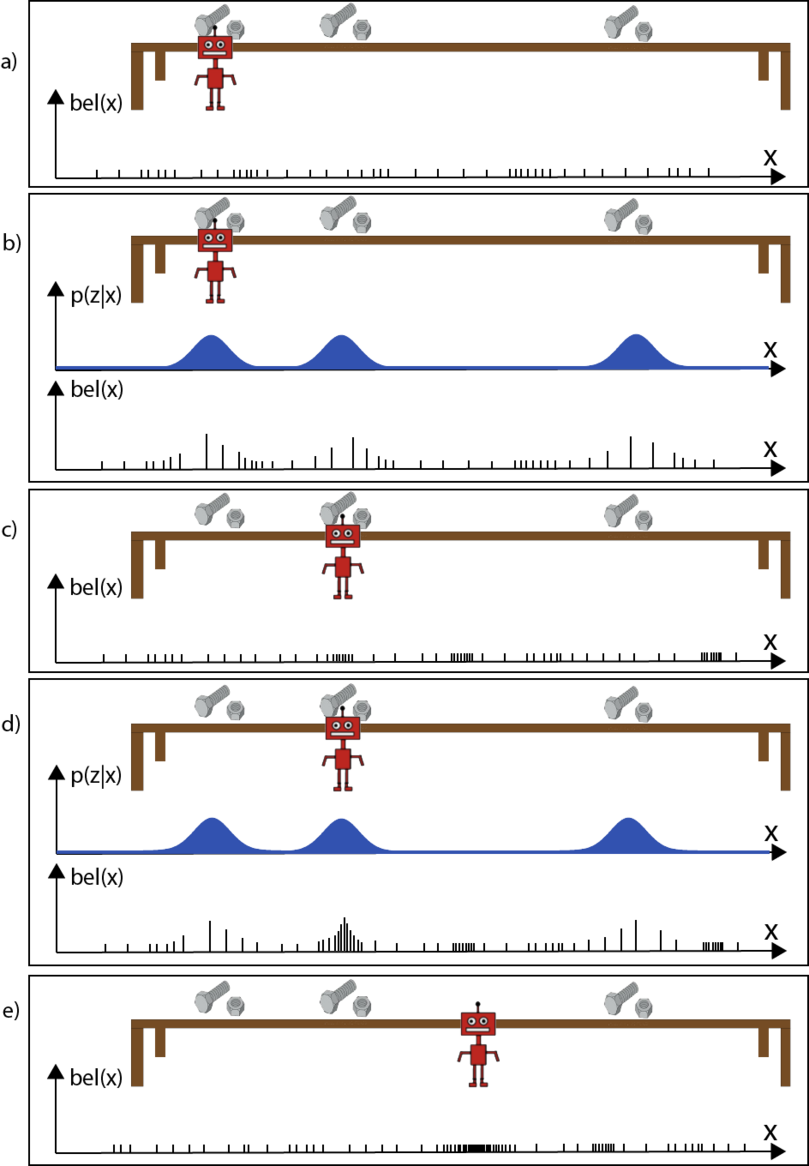
Fig. 19 Monte Carlo Localization. Vertical lines represent particles whose height represents the weight of the particle. p(z|x) is the measurement function. Figure inspired by Probabilistic Robotics.

• a. The robot starts in front of the first bolt. A set of particles are initialized in random positions throughout the state space. Notice that the particles have uniform initial weights.

• b. We weight the set of particles based on their nearness to the bolts using the measurement function.

• c. The robots moves from the first bolt to the second one, the motion model causes all particles to shift to the right. In this step, we also resample a new set of particles around the most likely positions from step b.

• d. Again, we weight the particles based on their nearness to the bolts, we can now see a significant concentration of the probability mass around the second bolt, where the robot actually is.

• e. The robot moves again and we resample particles around those highest weighted from part d. We can now see that the belief distribution is heavily concentrated around the true pose of the robot.

If you are feeling shaky about the MC localization algorithm, we recommend studying the diagram above until things start to make sense!

In localization_answers.md provide answers to the following questions:

Problem 1 - Localization Theory Questions

Q1- What is the advantage of particle filters relative to the Gaussian representation used by the Kalman filter?

Q2- Can Monte Carlo Localization approximate any distribution? If no, explain why? If yes, describe what controls the nature of approximation?