Our Localization Implementation

To complete our understanding of how we will implement a particle filter on the drone for localization, we need to address specific state transition and measurement models.

OpenCV and Features

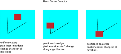
The drone’s primary sensor is its downward-facing camera. To process information from the camera, we will use a popular open source computer vision library called OpenCV. We can use opencv to extract features from an image. In computer vision, features are points in an image where we suspect there is something interesting going on. For a human, it is easy to identify corners, dots, textures, or whatever else might be interesting in an image. But a computer requires a precise definition of thing-ness in the image. A large body of literature in computer vision is dedicated to detecting and characterizing features, but in general, we define features as areas in an image where the pixel intensities change rapidly. In the following image, features are most likely to be extracted at the sharp corner in the line. Imagine looking at the scene through the red box as it moved around slightly in several directions starting in each of the three points shown below. Through which box would you see the scene change the most?

When we extract features from the drone’s camera feed, OpenCV will give us a keypoint and descriptor for each feature. The keypoint holds the (x,y) coordinate of the feature in the image frame. The descriptor holds information about the feature which can be used to uniquely identify it, commonly stored as a binary string.

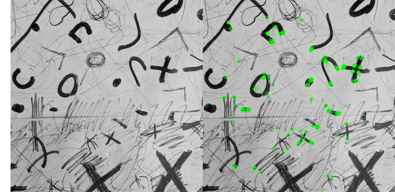
Fig. 20 An image taken on the drone’s camera, shown with and without plotting the coordinates of 200 features detected by ORB

The specific feature detector we will be using is called ORB.

See also

If you want to learn more about ORB, you may read more about it here .

Using OpenCV, we are able to perform some powerful manipulations on features. For example, panoramic image stitching can be achieved by matching feature descriptors from many overlapping images, and using their corresponding keypoints to precisely line up the images and produce a single contiguous scene.

We will use OpenCV features to implement both the motion (state transition) and measurement models for localization. We can find the movement of the drone for the motion update by measuring how far it moves between consecutive camera frames. This is done by matching the descriptors between two frames, then using their keypoint positions to compute a transformation between the frames. This transformation will give us an x, y, and yaw displacement between two frames. Note that this requires some overlap between two image frames.

To find the probability for each particle, we would like to measure the accuracy of the particle’s pose. We will do this by comparing the camera’s current image to the map of the drone’s environment. Remember, this is a localization algorithm, meaning that we have a map available beforehand. In our case, the map is an image of the area over which the drone will fly. We can match the descriptors from the current image to the descriptors in the map image, and compute the transformation between the sets of corresponding keypoints to obtain a global pose estimate. The probability that a given particle is the correct pose of the drone is proportional to the error between the global pose estimate and the particle’s pose.

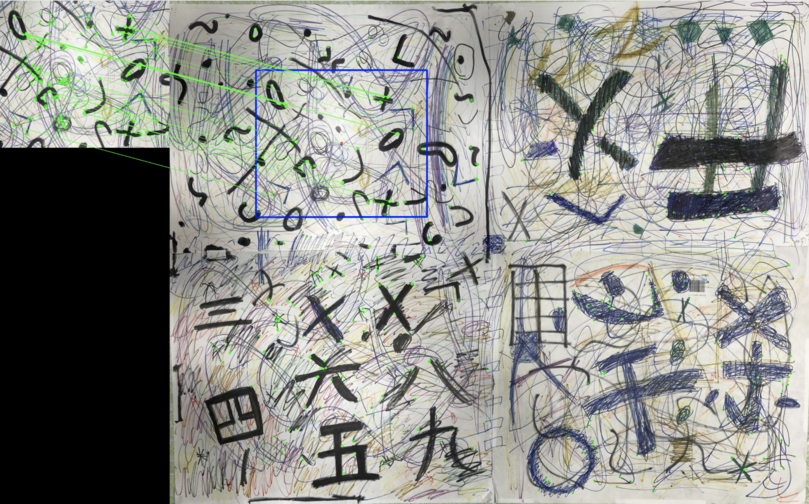
Fig. 21 Computing the transformation from the drone’s current view to the map in order to determine global pose

The following algorithm formulates precisely how we will use the ability visualized above to compute the global pose to weight the particles in MC localization. We observe features and attempt to match them to the map. If there enough matches, we compute the global pose of the drone, and compute q, the probability of the particle. q is equal to the product of the probabilities of the error between the particle’s pose and the computed global pose in x, y, and yaw.

\(\hspace{5mm} \textbf{Landmark Model Known Correspondence} \hspace{30mm}\\\) \(\hspace{5mm} \textbf{Measure}(\mathbf{c_t, x_t, m}) \hspace{30mm}\\\) \(\hspace{10mm} \mathbf{c \gets match(c_t,m)} \hspace{40mm}\\\) \(\hspace{10mm} \textbf{If} \mathbf{|c| \geq n} \hspace{30mm}\\\) \(\hspace{15mm} \mathbf{x,y,yaw=compute(c)} \hspace{30mm}\\\) \(\hspace{15mm} \mathbf{q=prob(x-x_t[0],\sigma_x^2) \cdot prob(y-x_t[1],\sigma_y^2) \cdot prob(yaw-x_t[3],\sigma_{yaw}^2)}\\\) \(\hspace{10mm} \textbf{Else} \hspace{50mm}\\\) \(\hspace{15mm} \mathbf{q=0} \hspace{50mm}\\\) \(\hspace{10mm} \textbf{Endif} \hspace{100mm}\\\) \(\hspace{5mm} \textbf{return q}\)

One final consideration for our implementation of MC Localization is how often to perform the motion and measurement updates. We ought to predict motion as often as possible to preserve the tracking of the drone as it flies. But the measurement update is more expensive than motion prediction, and doesn’t need to happen quite so often.

A naive solution is to perform updates after every set number of camera frames. But since we are already computing the distance between each frame, it is straightforward to implement a system which waits for the drone to move a certain distance before updating. This idea is known as a keyframe scheme and is useful in many scenarios when computations on every camera frame are not feasible. It will be useful later on in SLAM to have the threshold for distance between two keyframes equal to the length of the camera’s field of view, so we will implement such a system here.