2D UKF Design and Implementation

Fig. 15 2D UKF Height Estimates Visualized in the JavaScript Web Interface

It is time for you to design and implement a 2D UKF specific to the Duckiedrone! For the implementation, we will have you use the Python library FilterPy, which abstracts away most of the nitty-gritty math. If needed, you can refer to the FilterPy documentation and source code here.

Handin

Use this link to generate a Github repo for this project. Clone the directory to your computer git clone https://github.com/h2r/project-ukf-2020-yourGithubName.git This will create a new folder.

Commit and push your changes before the assignment is due. This will allow us to access the files you pushed to Github and grade them accordingly. If you commit and push after the assignment deadline, we will use your latest commit as your final submission, and you will be marked late.

cd project-ukf-2020-yourGithubName
git add -A
git commit -a -m 'some commit message. maybe handin, maybe update'
git push

Note that assignments will be graded anonymously, so please don’t put your name or any other identifying information on the files you hand in.

Design and Implement the 2D Filter

This part of the project has two deliverables in your repository, which are to be accessed and submitted via GitHub Classroom:

1. A \(\LaTeX\) PDF document ukf2d_written_solutions.pdf, generated from ukf2d_written_solutions.tex, with the answers to the UKF design and implementation questions.

2. Your implementation of the UKF written in the state_estimators/student_state_estimator_ukf_2d.py stencil code. In this stencil code file, we have placed TODO tags describing where you should write your solution code to the relevant problems.

In addition to implementing the UKF in code, we want you to learn about the design process, much of which occurs outside of the code that will run the UKF. Plus, we have some questions we want you to answer in writing to demonstrate your understanding of the UKF. Hence, you will be writing up some of your solutions in \(\LaTeX\). We are having you write solutions in \(\LaTeX\) because it will in particular enable you to write out some of the UKF math in a clear (and visually appealing!) format. In these documents, please try to follow our math notation wherever applicable.

Task: From your repository, open up the ukf2d_written_solutions.tex file in your favorite \(\LaTeX\) editor. This could be in Overleaf, your Brown CS department account, or locally on your own computer. Before submitting your document, please make sure it is compiled into a PDF. If you are having trouble with \(\LaTeX\), please seek out the help of a TA.

State Vector

For this part of the project, we are going to track the drone’s position and velocity along the \(z\)-axis:

\[\begin{split}\mathbf{x}_t=\begin{bmatrix} z \\ \dot z \end{bmatrix}\end{split}\]

State Transition Function

For this UKF along the \(z\)-axis, your state transition function will take into account a control input \(\mathbf{u}\) defined as follows:

\[\mathbf{u}_t=\begin{bmatrix} \ddot z \end{bmatrix}\]

\(\ddot z\) is the linear acceleration reading along the \(z\)-axis provided by the IMU.

Task (Written Section 1.2.2): Implement the state transition function \(g(\mathbf{x}_{t-\Delta t}, \mathbf{u}_t, \Delta t)\) by filling in the template given in Section 1.2.2 of ukf2d_written_solutions.tex with the correct values to propagate the current state estimate forward in time. Remember that for the drone, this involves kinematics (hint: use the constant acceleration kinematics equations). Since there is a notion of transitioning the state from the previous time step, this function will involve the variable \(\Delta t\).

Task: Translate the state transition function into Python by filling in the state_transition_function() method in state_estimators/student_state_estimator_ukf_2d.py. Follow the “TODO”s there. Note the function’s type signature for the inputs and outputs.

Measurement Function

At this stage, we are only considering the range reading from the IR sensor for the measurement update step of the UKF, so your measurement vector \(\mathbf{z}_t\) will be the following:

\[\mathbf{z}_t = \begin{bmatrix} r \end{bmatrix}\]

Task (Written Section 1.3.2): In ukf2d_written_solutions.tex, implement the measurement function \(h(\mathbf{\bar x}_t)\) to transform the prior state estimate into measurement space. For this model’s state vector and measurement vector, \(h(\mathbf{\bar x}_t)\) can be implemented as a \(1 \times 2\) matrix that is multiplied with the \(2 \times 1\) state vector, outputting a \(1 \times 1\) matrix: the same dimension as the measurement vector \(\mathbf{z}_t\), which allows for the computation of the residual.

Task: As before, translate the measurement function into code, this time by filling in the measurement_function() method. Follow the “TODO”s there. Note the function’s type signature for the inputs and outputs.

Process Noise and Measurement Covariance Matrices

The process noise covariance matrix \(\mathbf{Q}_t\) represents how uncertain we are about our motion model. It needs to be determined for the prediction step, but you do not need to determine this yourself, as this matrix can be notoriously difficult to ascertain. Feasible values for the elements of \(\mathbf{Q}_t\) are provided in the code.

On the other hand, the measurement noise covariance matrix \(\mathbf{R}_t\) has a more tangible meaning: it represents the variance in our sensor readings, along with covariances if sensor readings are correlated. For our 1D measurement vector, this matrix just contains the variance of the IR sensor.

The interplay between \(\mathbf{Q}_t\) and \(\mathbf{R}_t\) dictates the value of the Kalman gain \(\mathbf{K}_t\), which scales our estimate between the prediction and the measurement.

Task: Characterize the noise in the IR sensor by experimentally collecting data from your drone in a stationary setup and computing its variance. To do so, prop the drone up so that it is stationary and its IR sensor is about 0.3 m from the ground, pointing down, unobstructed. To collect the range data, execute the following commands on your drone:

Navigate to pidrone_pkg and start the code:

$ roscd pidrone_pkg
$ ./start.sh

After navigating to a free screen, echo the infrared ROS topic and extract just the range value. To automatically log a lot of IR range readings, you must redirect standard output to a file like so:

$ rostopic echo /pidrone/infrared/range > ir_data.txt

We have provided a script ir_sample_variance_calculation.py that reads in the range readings from the file (so make sure this file is named ir_data.txt and is in the same directory as ir_sample_variance_calculation.py), computes the sample variance, and plots the distribution of readings using matplotlib. If you want to run this on your drone, then you will have to ensure that your ssh client has the capability to view pop-up GUI windows in order to view the plot. If you have XQuartz installed on your base station, for example, then this should allow you to run ssh -Y [email protected]. Otherwise, you can run this script on a computer that has Python, matplotlib, and numpy installed.

Your plot should look somewhat Gaussian, as in Fig. 16.

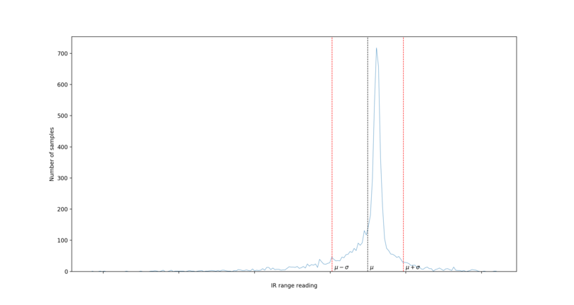
Fig. 16 Sample Distribution of Infrared Range Data

When running ir_sample_variance_calculation.py, you can pass in command-line arguments of -l to plot a line chart instead of a bar chart and -n followed by a positive integer to indicate the number of intervals to use for the histogram (defaults to 100 intervals).

Task (Written Section 1.3.3): Record the resulting sample variance value in ukf2d_written_solutions.tex. Also include an image of your histogram in ukf2d_written_solutions.tex.

Task: Enter this sample variance value into the code for self.ukf.R in the initialize_ukf_matrices() method.

Initialize the Filter

Before the UKF can begin its routine of predicting and updating state estimates, it must be initialized with values for the state estimate \(\mathbf{x}_t\) and state covariance matrix \(\mathbf{P}_t\), as the first prediction call will rely on propagating these estimates forward in time. There is no set way to initialize the filter, but one common approach is to simply take the first measurements that the system receives and treat them as the best estimate of the state until we have estimates for each variable.

Task: For your drone, you want to wait until the first IR reading comes in and then set the corresponding \(z\) position value equal to this measurement. This only accounts for one of the two state variables. For now, initialize \(\dot z=0 \text{ m/s}\). Go ahead and implement this state estimate initialization in code in the ir_data_callback() method, which gets called each time this ROS node receives a message published by the IR sensor.

Task: In addition to initializing the state estimate, you must initialize the time value corresponding to the state estimate. We provide a method initialize_input_time() that accomplishes this, but you must call it in the appropriate location.

Another aspect of the filter that can be initialized upon the first receipt of a measurement is the state covariance matrix \(\mathbf{P}_t\). How do we know what values to use for this initialization? Again, this is a design decision that can vary by application. We can directly use the variance of the IR sensor to estimate an initial variance for the height estimate. We won’t worry about initializing the velocity variance or the covariances. If we always knew that we were going to start the filter while the drone is at rest, then we could confidently initialize velocity to 0 and assign a low variance to this estimate.

Task: Initialize the \(\mathbf{P}_t\) matrix in the ir_data_callback() method with the variance of the IR sensor for the variance of the \(z\) position estimate. FilterPy initializes instance variables for you, but you should assign these variables initial values. You can refer to the FilterPy documentation to figure out what variable names to use.

Task (Written Section 2.1): How else could you initialize the estimate for \(\dot z\) given the raw range readings from the IR sensor? Recall that the range readings are an estimate for \(z\), and you can differentiate \(z\) to get \(\dot z\). Describe in ukf2d_written_solutions.tex what you would do and the potential pros and cons of your approach. Do not implement this in code.

It is unlikely that the filter initialization will be perfect. Fret not—the Kalman Filter can handle poor initial conditions and eventually still converge to an accurate state estimate. Once your predict-update loop is written, we will be testing out the impact of filter initialization.

Asynchronous Inputs

The traditional Kalman Filter is described as a loop alternating between predictions and measurement updates. In the real world, however, we might receive control inputs more frequently than we receive measurement updates; as such, instead of throwing away information, we would prefer to perform multiple consecutive predictions. Additionally, our inputs (i.e., control inputs and sensor data) generally arrive asynchronously, yet the traditional Kalman Filter algorithm has the prediction and update steps happen at the same point in time. Furthermore, the sample rates of our inputs are typically not constant, and so we cannot design our filter to be time invariant. These are all problems that should be considered when transitioning from the theoretical algorithm to the practical application.

Task (Written Section 2.2): Describe why, in a real-world Kalman Filter implementation, it generally makes sense to be able to perform multiple consecutive predictions before performing a new measurement update, whereas it does not make sense algorithmically to perform multiple consecutive measurement updates before forming a new prediction. It might be helpful to think about the differences between what happens to the state estimate in the prediction versus the update step. Write your answer in ukf2d_written_solutions.tex.

Task: Implement the predicting and updating of your UKF, keeping in mind the issue of asynchronous inputs. These steps will occur in two ROS subscriber callbacks: 1) imu_data_callback when an IMU control input is received and 2) ir_data_callback when an IR measurement is received. Remember that we want to perform a prediction not only when we receive a new control input but also when we receive a new measurement in order to propagate the state estimate forward to the time of the measurement. One way to do this prediction without a new control input is to assume that the control input remains the same as last time (which is what we suggest); another potential approach might be to not include a control input in those instances (i.e., set it to zeros). The method for our FilterPy UKF object that you want to use to perform the prediction is self.ukf.predict(), which takes in a keyword argument dt that is the time step since the last state estimate and a keyword argument u, corresponding to the argument u of state_transition_function(), that is a NumPy array with the control input(s). The method to do a measurement update is self.ukf.update(), which requires a positional argument consisting of a measurement vector as a NumPy array. Call self.publish_current_state() at the end of each callback to publish the new state estimate to a ROS topic.

Note that these callbacks get called in new threads; therefore, there is the potential for collisions when, say, both IMU and IR data come in almost at the same time and one thread has not had the opportunity to finish its UKF computations. We don’t want both threads trying to simultaneously alter the values of certain variables, such as the \(\mathbf{P}_t\) matrix when doing a prediction, as this can cause the filter to output nonsensical results and break. Therefore, we have implemented a simple callback blocking scheme—using the self.in_callback variable—that ignores a new callback if another callback is going on, essentially dropping packets if there are collisions. While this may not be the optimal or most stable way to handle the issue (one could imagine the IMU callback, for example, always blocking the IR callback and hence preventing measurement updates), it at least gets rid of the errors that would occur with collisions. If you so desire, feel free to implement your own callback management system that perhaps balances the time allocated to different callbacks.

Tune and Test the Filter

In this problem, you will be testing your UKF that you have implemented thus far. You will start by testing on simulated drone data. We have set up the simulation to publish its data on ROS topics so that your UKF program interfaces with the drone’s ROS environment and will be able to be applied directly to real, live data coming from the drone during flight. The output from the UKF can be evaluated in the JavaScript web interface (see pidrone_pkg/web/index.html).

In Simulation

To run your UKF with simulated drone data, you first have to make sure that your package is in the ~/ws/src directory on your drone. Your package has a unique name, so you will need to modify some files. There are two places near the top of package.xml where you should replace pidrone_project2_ukf with your repo name, and similarly there is one place near the top of the CMakeLists.txt file where you should do the same. Then, in ~/ws, run catkin_make to build your package. By running this command, you will be able to run ROS and access nodes from your package. If you experience issues with catkin, please do not hesitate to reach out to the TAs.

In order to test your UKF within our software stack, navigate to the file in pidrone_pkg/scripts called state_estimator.py and edit the line that assigns a value to student_project_pkg_dir, instead inserting your project repo name project-ukf-2020-yourGithubName.

Next, run ROS as usual with the ./staart_pidrone_code.sh file in the pidrone_pkg. Upon start-up, go ahead and terminate the IR and flight controller nodes, as these would conflict with the drone simulator’s simulated sensors. In the state estimator screen, terminate the current process and then run the following command:

python state_estimator.py --student --primary ukf2d --others simulator --ir_var IR_VARIANCE_ESTIMATE

with your computed estimate of your IR sensor’s variance that you used to determine the \(\mathbf{R}_t\) matrix in your UKF in place of IR_VARIANCE_ESTIMATE. This command will automatically run your 2D UKF as the primary state estimator, along with the drone simulator. The EMA filter will also be run automatically with the 2D UKF, since the 2D UKF does not provide a very complete state vector in three-dimensional flight scenarios. This will also by default allow you to compare the output of your UKF to the EMA filter on altitude. Note the --student flag, which ensures that your UKF script is run.

Now in the web interface, once you connect to your drone, you should see four curves in the Standard View of the Height Readings chart as in Fig. 17.

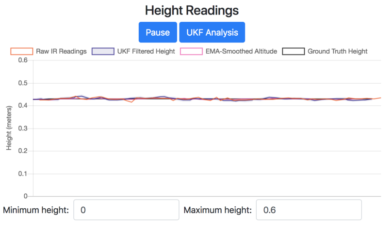
Fig. 17 Standard View of the Height Readings Chart with Drone Simulated Data

1. Raw IR Readings: the orange curve that shows the drone simulator’s simulated noisy IR readings

2. UKF Filtered Height: the blue curve that shows your UKF’s height estimates, along with a shaded region indicating plus and minus one standard deviation, which is derived from the \(z\) position variance in the covariance matrix

3. EMA-Smoothed Altitude: the pink curve that shows the EMA filter’s estimates

4. Ground Truth Height: the black curve that is the simulated drone’s actual height that we are trying to track with the UKF

If you click on the UKF Analysis button, the chart will change over to reveal different datasets, shown in Fig. 18.

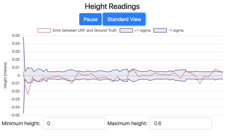
Fig. 18 UKF Analysis View of the Height Readings Chart with Drone Simulated Data

With this chart, we can analyze the performance of the UKF. The orange curve represents the error between the UKF and ground truth from the simulation; the closer to zero this value, the better the UKF estimates are tracking the actual altitude of the simulated drone. The blue shaded region indicates plus and minus one standard deviation of the UKF’s \(z\) position estimates. If the system is indeed behaving in a nice Gaussian manner and the UKF is well tuned, then we expect to see about 68% of the points in the orange dataset lying in the blue shaded region. Also note that on the left side of Fig. 18, the standard deviation and error start off relatively high; this is because the filter is starting out, improving its estimates from initial values.

If you are seeing that your UKF altitude estimates are lagging significantly behind the simulated data in the Height Readings chart, then this is likely due to computation overhead. The UKF takes time to compute, and if it tries to compute a prediction and/or update for each sensor value that it receives, it can sometimes fall behind real time. In this case, you should run the state estimator with the IR and IMU data streams throttled:

python state_estimator.py --student --primary ukf2d --others simulator --ir_var IR_VARIANCE_ESTIMATE --ir_throttled --imu_throttled

Make sure your UKF is producing reasonable outputs that seem to track ground truth pretty well. In the UKF Analytics view of the chart, you should see about two-thirds of the points in the error dataset lying within one standard deviation, based on your UKF’s state covariance, relative to ground truth.

To test out your UKF’s robustness in the face of poor initialization, you can compare how long it takes the state estimates to converge to accurate values with good initial conditions and with poor initial conditions. You do not have to report or hand in anything for this task; it is just for your understanding of the capabilities of the UKF.

Manually Moving the Drone Up and Down

Next, you will step out of the realm of simulation and test your UKF on your drone, manually moving it along the vertical axis to test out the response you get with your IR sensor. For this step, the command you want to use is:

python state_estimator.py --student --primary ukf2d

with the --ir_throttled and --imu_throttled flags as needed. You want to make sure your IR sensor and flight controller nodes are actually running. First, quit any existing screens, then calibrate your accelerometer with:

roscd pidrone_pkg
python scripts/calibrateAcc.py

Debugging Task: Test out your UKF by moving your drone up and down and examining the Height Readings chart. Does it behave as you expect? Does the estimated height seem to have more or less noise than the raw IR sensor reading? If there are unexpected deviations or spikes from the measurements, consider why this might be, especially in comparison to the results you saw when running the UKF in simulation. A possible cause is that the prediction step without a measurement update is not being modeled well or is getting poor/noisy control inputs to the point where the process noise that we assigned was too low. Try tuning the scalar that multiplies the values of the \(\mathbf{Q}_t\) matrix self.ukf.Q in the initialize_ukf_matrices() method to better reflect the variance of the process. You should see a greater standard deviation as well as smaller spikes in the estimates.

Another aspect that you should consider is the prediction that occurs in your IMU callback. Note that the unthrottled sample rate of the IR sensor is around 80 Hz, while the IMU only comes in at about 30 Hz. Therefore, the control input is being changed less frequently than the predictions and measurement updates occur in the IR callback. While in the Asynchronous Inputs section we indicated that you should do a prediction whenever you get a new control input, in this application, it might make sense to save computation and only do predictions right before measurement updates. Plus, the accelerometers are noisy, and it can be difficult in a discrete domain to integrate these accelerations and expect accurate position estimates reported before including the measurement update. To keep our estimates reasonable, we can wait for the measurement update step to fuse the noisy prior prediction with the new measurement—and since this step can actually occur more frequently than the control input, we can maintain good measurement-informed estimates while saving on prediction computation. To simplify the problem, we can move the prediction and update out of a sensor callback and in its own loop in the main thread of the program.

Task: Modify your UKF to only do predictions and updates in a loop in the main thread of your program, using rospy.Rate(self.loop_hz) to regulate the rate at which the UKF tries running (feel free to look up documentation on how to use rospy.Rate()). You will want to store the data that come in from the IMU and IR sensor in instance variables that you can use in your main loop. Note that you should now use the -hz flag followed by a number (defaults to 30), rather than the various sensor throttle flags, to alter the rate of your UKF. Visually compare your UKF output to the EMA output.

Task: Visually compare the UKF output with and without the IMU running. You should notice a difference in how well/quickly the UKF tracks the measurements when there is no control input to better inform the prediction step.

Task (Written Section 2.3): In ukf2d_written_solutions.tex, describe how a (well-tuned) Kalman Filter outperforms an exponential moving average (EMA) filter applied to raw sensor data. Test this out by moving your drone up and down and comparing the UKF and EMA estimates. Once your UKF seems to outperform the EMA, attach an image of the Height Readings graph to your ukf2d_written_solutions.tex document showing this difference between your UKF and the EMA, and briefly describe the different features.

In Flight

It’s time to fly your drone with the UKF providing it with real-time filtered estimates of its position and velocity along the \(z\)-axis.

Task: Fly your drone while running:

python state_estimator.py --student --primary ukf2d

with the -hz flag as needed. Evaluate its performance using the web interface as you did for the manual motion testing.