Part 2: Affine Transformations
Contents
Part 2: Affine Transformations#
Background Information#
In order to estimate the Duckiedrone’s position (a 2-dimensional column vector \(v = [x \; y]^T\)) using the camera, you will need to use affine transformations. An affine transformation \(f: \mathbb{R}^n \to \mathbb{R}^m\) is any transformation of the form \(v \to Av + b\), where \(A \in \mathbb{R}^{m \times n}\) and \(b \in \mathbb{R}^m\). The affine transformations we are interested in are rotation, scale, and translation in two dimensions. So, the affine transformations we will look at will map vectors in \(\mathbb{R}^2\) to other vectors in \(\mathbb{R}^2\).
Let’s first look at rotation. We can rotate a column vector \(v \in \mathbb{R}^2\) about the origin by the angle \(\theta\) by premultiplying it by the following matrix:
Let’s look at an example. Below we have the vector \([1, 2]^T\). To rotate the vector by \(\theta=\frac{2\pi}{3}\), we pre-multiply the vector by the rotation matrix:
A graphical representation of the transformation is shown below. The vector \([1, 2]^T\) is rotated \(\frac{2\pi}{3}\) about the origin to get the vector \([-2.232, -0.134]^T\)
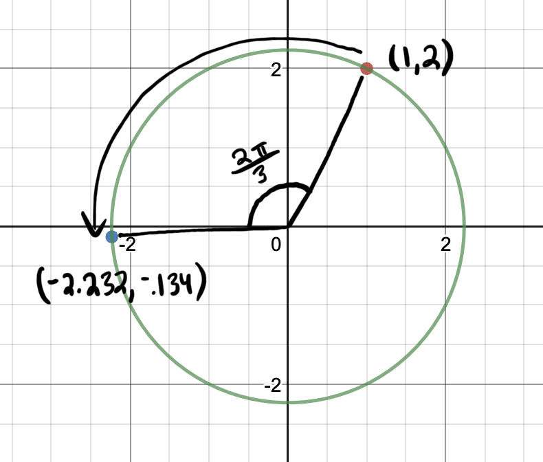
Fig. 1 Rotating one point about the origin#
Next, let’s look at how scale is represented. We can scale a vector \(v \in \mathbb{R}^2\) by a scale factor \(s\) by pre-multiplying it by the following matrix:
We can scale a single point \([1, 2]^T\) by a factor of .5 as shown below:
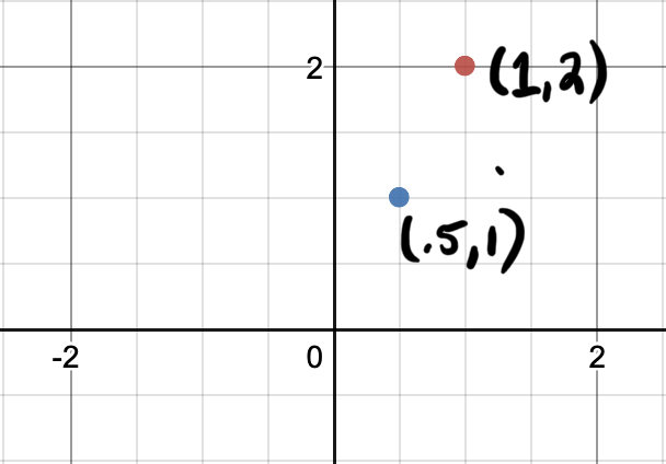
Fig. 2 Scaling one point#
When discussing scaling, it is helpful to consider multiple vectors, rather than a single vector. Let’s look at all the points on a rectangle and multiply each of them by the scale matrix individually to see the effect of scaling by a factor of .5:
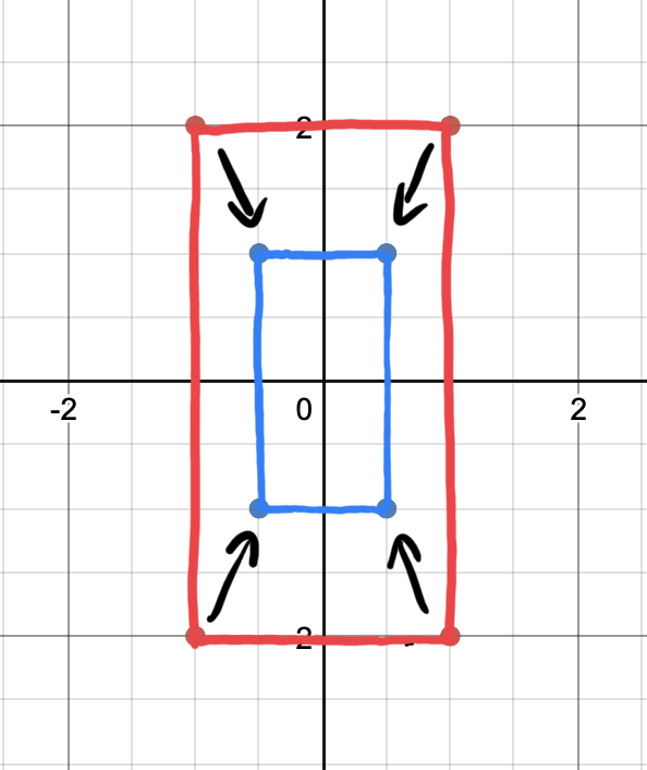
Fig. 3 Scaling multiple points#
Now we can see that the rectangle was scaled by a factor of .5.
What about translation? Remember that an affine transformation is of the form \(v \to Av + b\). You may have noticed that rotation and scale are represented by only a matrix \(A\), with the vector \(b\) effectively equal to 0. We could represent translation by simply adding a vector \(b = [dx \; dy]^T\) to our vector \(v\). However, it would be convenient if we could represent all of our transformations as matrices, and then obtain a single transformation matrix that scales, rotates, and translates a vector all at once. We could not achieve such a representation if we represent translation by adding a vector.
So how do we represent translation (moving \(dx\) in the \(x\) direction and \(dy\) in the \(y\) direction) with a matrix? First, we append a 1 to the end of \(v\) to get \(v' = [x, y, 1]^T\). Then, we premultiply \(v'\) by the following matrix:
Even though we are representing our \(x\) and \(y\) positions with a 3-dimensional vector, we are only ever interested in the first two elements, which represent our \(x\) and \(y\) positions. The third element of \(v'\) is always equal to 1. Notice how pre-multiplying \(v'\) by this matrix adds \(dx\) to \(x\) and \(dy\) to \(y\). $\( \begin{bmatrix} 1 & 0 & dx\\ 0 & 1 & dy\\ 0 & 0 & 1\\ \end{bmatrix} \begin{bmatrix} x \\ y \\ 1 \\ \end{bmatrix} = \begin{bmatrix} x + dx \\ y + dy\\ 1 \\ \end{bmatrix} \)$
So this matrix is exactly what we want!
As a final note, we need to modify our scale and rotation matrices slightly in order to use them with \(v'\) rather than \(v\). A summary of the relevant affine transforms is below with these changes to the scale and rotation matrices.
Estimating Position on the Duckiedrone#
Now that we know how rotation, scale, and translation are represented as matrices, let’s look at how you will be using these matrices in the sensors project.
To estimate your drone’s position, you will be using a function from OpenCV called
estimateRigidTransform. This function takes in two images \(I_1\) and \(I_2\) and a boolean \(B\). The function returns a matrix estimating the affine transform that would turn the first image into the second image. The boolean \(B\) indicates whether you want to estimate the affect of shearing on the image, which is another affine transform. We don’t want this, so we set \(B\) to False.
estimateRigidTransform returns a matrix in the form of:
This matrix should look familiar, but it is slightly different from the matrices we have seen in this section. Let \(R\), \(S\), and \(T\) be the rotation, scale, and translation matrices from the above summary box. Then, \(E\) is the same as \(TRS\), where the bottom row of \(TRS\) is removed. You can think of \(E\) as a matrix that first scales a vector \(u = [x, y, 1]^T\) by a factor of \(s\), then rotates it by \(\theta\), then translates it by \(dx\) in the \(x\) direction and \(dy\) in the \(y\) direction, and then removes the 1 appended to the end of the vector to output \(u' = [x', y']\).
Wow that was a lot of reading! Now on to the questions…
Questions#
Your Duckiedrone is flying over a highly textured planar surface. The Duckiedrone’s current \(x\) position is \(x_0\), its current \(y\) position is \(y_0\), and its current yaw is \(\phi_0\). Using the Raspberry Pi Camera, you take a picture of the highly textured planar surface with the Duckiedrone in this state. You move the Duckiedrone to a different state (\(x_1\) is your \(x\) position, \(y_1\) is your \(y\) position, and \(\phi_1\) is your yaw) and then take a picture of the highly textured planar surface using the Raspberry Pi Camera. You give these pictures to
esimateRigidTransformand it returns a matrix \(E\) in the form shown above.Write expressions for \(x_1\), \(y_1\), and \(\phi_1\). Your answers should be in terms of \(x_0\), \(y_0\), \(\phi_0\), and the elements of \(E\). Assume that the Duckiedrone is initially is located at the origin and aligned with the axes of the global coordinate system.
Hint 1: Your solution does not have to involve matrix multiplication or other matrix operations. Feel free to pick out specific elements of the matrix using normal 0-indexing, i.e. \(E[0][2]\).
Hint 2: Use the function arctan2 in some way to compute the yaw.