PID Controllers generalities

Introduction

A PID (proportional, integral, derivative) controller is a control algorithm extensively used in industrial control systems to generate a control signal based on error. The error is calculated by the difference between a desired setpoint value, and a measured process variable. The goal of the controller is to minimize this error by applying a correction to the system through adjustment of a control variable. The value of the control variable is determined by three control terms: a proportional term, integral term, and derivative term.

Characteristics of the Controller

Key Terms and Definitions

• Process Variable: The parameter of the system that is being monitored and controlled.

• Setpoint: The desired value of the process variable.

• Control Variable/Manipulated Variable: The output of the controller that serves as input to the system in order to minimize error between the setpoint and the process variable.

• Steady-State Value: The final value of the process variable as time goes to infinity.

• Steady-State Error: The difference between the setpoint and the steady-state value.

• Rise Time: The time required for the process variable to rise from 10 percent to 90 percent of the steady-state value.

• Settling Time: The time required for the process variable to settle within a certain percentage of the steady-state value.

• Overshoot: The amount the process variable exceeds the setpoint (expressed as a percentage).

General Algorithm

The error of the system \(e(t)\), is calculated as the difference between the setpoint \(r(t)\) and the process variable \(y(t)\). That is:

\[e(t) = r(t) - y(t)\]

The controller aims to minimize the rise time and settling time of the system, while eliminating steady-state error and maximizing stability (no unbounded oscillations in the process variable). It does so by changing the control variable \(u(t)\) based on three control terms.

Proportional Term

The first control term is the proportional term, which produces an output that is proportional to the calculated error:

\[P = K_pe(t)\]

The magnitude of the proportional response is dependent upon \(K_p\), which is the proportional gain constant. A higher proportional gain constant indicates a greater change in the controller’s output in response to the system’s error.

Integral Term

The second control term is the integral term, which accounts for the accumulated error of the system over time. The output produced is comprised of the sum of the instantaneous error over time multiplied by the integral gain constant \(K_i\):

\[I = K_i\int_0^t\!e(\tau)\,\mathrm{d}\tau\]

Derivative Term

The final control term is the derivative term, which is determined by the rate of change of the system’s error over time multiplied by the derivative gain constant \(K_d\):

\[D = K_d\frac{de(t)}{dt}\]

Overall Control Function

The overall control function can be expressed as the sum of the proportional, integral, and derivative terms:

\[u(t) = K_pe(t) + K_i\int_0^t\!e(\tau)\,\mathrm{d}\tau + K_d\frac{de(t)}{dt}\]

In practice, the discretized form of the control function may be more suitable for implementation:

\[u(t) = K_pe(t_k) + K_i\sum_{i=0}^k e(t_i)\Delta t + K_d\frac{e(t_k)-e(t_{k-1})}{\Delta t}\]

The figure below summarizes the inclusion of a PID controller within a basic control loop.

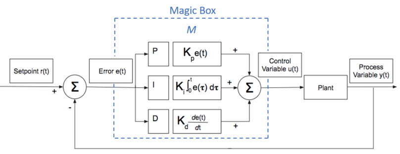
Fig. 8 PID Controller Block Diagram

Tuning

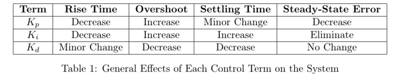
Tuning a PID controller refers to setting the control parameters \(K_p\), \(K_i\), and \(K_d\) to optimal values in order to obtain the ideal control response. After understanding the general effects of each control term on the control response, tuning can be accomplished through trial-and-error or by other specialized tuning schemes, such as the Ziegler-Nichols tuning method. A graph of the process variable or system error can display the effects of the controller terms on the system; the control parameters can then be modified appropriately to optimize the control response. Although the independent effects of each parameter are explained below, the three control terms may be correlated and so changing one parameter may impact the influence of another. The general effects of each term are therefore useful as reference, but the actual effects will vary depending on the specific control system.

Effects of \(K_p\)

For a given level of error, increasing \(K_p\) will proportionally increase the control output. This causes the system to react more quickly (thereby decreasing the rise time and the settling time by a small amount). Even so, setting the proportional gain too high could cause massive overshoot, which in turn could destabilize the system. Increasing \(K_p\) also has the effect of decreasing the steady-state error. However, as the value of the process variable approaches the setpoint and the error decreases, the proportional term will also decrease. As a result, with a P-controller (a controller with only the proportional term), the process variable will asymptotically approach the setpoint, but will never quite reach it. Thus, a P-controller cannot be used to completely eliminate steady-state error.

Effects of \(K_i\)

The integral term takes into account past error, as well as the duration of the error. If error persists for a long time, the integral term will continue to accumulate and will eventually drive the error down. This has the effect of reducing and eliminating steady-state error. However, the build-up of error can cause the value of the process variable to overshoot, which can increase the settling time of the system, though it decreases the rise time.

Effects of \(K_d\)

By calculating the instantaneous rate of change of the system’s error and using this slope for linear extrapolation, the derivative term anticipates future error. While the proportional and integral terms both act to move the process variable to the setpoint, the derivative term seeks to dampen their efforts and decrease the amount the system overshoots in response to a large change in error (which would greatly affect the magnitude of the proportional and integral contributions to the overall control output). If set at an appropriate level, the derivative term reduces oscillations, which decreases the settling time and improves the stability of the system. The derivative term has negligible effects on steady-state error and only decreases the rise time by a minor amount.

Summary of Control Terms

Fig. 9 General Effects of Control Terms

Ziegler-Nichols Closed-Loop Tuning Method

Ziegler and Nichols [] developed two techniques for tuning PID controllers, a closed-loop tuning method and an open-loop tuning method. With the closed-loop tuning method, the PID controller is initially turned into a P controller with \(K_p\) set to zero. \(K_p\) is slowly increased until the system exhibits stable oscillatory behavior, at which point it is denoted \(K_u\), the ultimate or critical gain. As such, \(K_u\) should be the smallest \(K_p\) value that causes the control loop to have regular oscillations. The ultimate or critical period \(T_u\) of the oscillations needs to be measured. Then, using the constants determined experimentally by Ziegler and Nichols, the controller gain values can be computed as follows:

\[ K_p = 0.6K_u \]

\[ K_i = 2K_p / (T_u) \]

\[ K_d = K_p(T_u) / 8 \]

Although the Ziegler-Nichols method may yield initial tuning values that work relatively well, the system’s control loop can be tuned further by adjusting the controller gain values based on the general effects of each control term as explained above.

Potential Problems

In real-world applications, the PID controller exhibits issues that require modifications to the general algorithm. In certain situations, one may find that a P-Controller, PD-Controller (eliminating the integral term), or a PI-Controller (eliminating the derivative term) are more advantageous controllers for the system. Alternatively, different techniques can be employed to counteract the problems that may affect the usability of a control term.

Integral Windup

Integral wind-up occurs when, due to a large change in setpoint, the control output causes the system’s actuator to become saturated. At this point, the integrated error between the process variable and the setpoint will continue to grow (because the actuator is at its limit and cannot drive the process variable any closer to the setpoint). In turn, the control output will continue to grow and will no longer have any effect on the system. When the setpoint finally changes and the error changes sign (meaning the new setpoint is now below the value of the process variable), the integral term will take a while to “unwind” all of the error that it has accumulated before producing a reverse control action that will move the process variable in the correct direction towards the setpoint.

There exist numerous ways to address integral wind-up. One way is to keep the integral term within predefined upper and lower bounds. Another way is to set the integral term to zero if the control output will cause the system’s actuator to saturate. Yet another way is to reduce the integral term by a constant multiplied by the difference between the actual output and the commanded output. If the actuator is not saturated, then the difference between the actual and commanded output will be zero and will not affect the integral term. If the actuator is saturated, then the additional feedback in the control loop will drive the commanded output closer to the saturation limit. If the setpoint changes and causes the error to change sign, then the integral term will not need to unwind in order to produce an appropriate control action. Setpoint ramping — in which the setpoint is increased or decreased incrementally to reach the desired value — may also help prevent integral wind-up.

Derivative Noise

Since the derivative term is proportional to the change in error, it is consequently highly sensitive to noise (which would produce drastic changes in error). Using a low-pass filter on the derivative term, or finding the derivative of the process variable (as opposed to the error), or taking a weighted mean of previous derivative terms could help ensure that high-frequency noise does not cause the derivative term to adversely affect the control output.

Cascaded Controllers

When multiple measurements can be used to control a single process variable, these measurements can be combined using a cascaded PID controller. In cascaded PID control, two PID controllers are used conjointly to yield a better control response. The output of the PID controller for the outer control loop determines the setpoint for the PID controller of the inner control loop. The outer loop controller controls the primary process variable of the system, while the inner loop controller controls a system parameter that tends to change more rapidly in order to minimize the error of the outer control loop. The two controllers have separate tuning values, which can be optimized for the part of the system that they control. This enables an overall better control response for the system as a whole.

High-Level Description of the Duckiedrone PID Stack

The drone platform utilizes a number of PID controllers to autonomously control its motion. The standard PID class implements the discrete version of the ideal PID control function. The control output returned is the sum of the proportional, integral, and derivative terms, as well as an offset constant term, which is the base control output before being corrected in response to the calculated error. A specified control range keeps the control output within predefined bounds.

Cascaded Position and Velocity Controllers

The flight command for the drone consists of four pulse-width modulation (pwm) values that are sent to the flight controller and translated into motor speeds to set the drone’s roll, pitch, yaw, and throttle, respectively. When the drone attempts to hover with zero velocity, or when a velocity command is sent from the web interface, the error between the commanded velocity and the actual velocity of the drone (determined by optical flow) is calculated. The x-velocity error serves as input to the roll PID controllers and the y-velocity error serves as input to the pitch PID controllers. For the throttle PID controllers, the z-position error is used as input. The z-velocity error is not used because the actual z-position of the drone is directly measured by the infrared sensor, and is thus easier to control, while the camera estimation of the z-velocity is not as accurate. The output of each controller is then used to set the roll, pitch, and throttle commands to achieve the desired velocity.

To accomplish position hold on the drone, cascaded PID controllers are utilized. The outer control loop is concerned with the position of the drone, and the inner control loop changes the velocity of the drone in order to attain the desired position. The two position PID controllers (one for front-back planar motion and the other for left-right planar motion) each calculate a setpoint velocity based on position error, which serves as input to the velocity PID controller. The roll, pitch, and throttle PID controllers then compute the appropriate flight commands based on the difference between the current velocity and this setpoint velocity.

Low and High Integral Terms

The drone requires two PID controllers to control each of its roll, pitch, and throttle. One controller has a fast-changing integral term with a high \(K_i\) value, while the other controller has a slow-changing integral term with a low \(K_i\) value. The inclusion of the low integral controller is intended to adjust for systemic sources of error, such as poor weight distribution or a damaged propeller. If the magnitude of the calculated velocity error is below a certain threshold, the flight command is set to the control output of its low integral controller and the integral term of its high integral controller is reset to zero. This helps to prevent integral wind-up for the high integral controller (the throttle PID controllers also use an integral term control range to bound the the value of the integral term and prevent wind-up). If the calculated velocity error is above the specified threshold, it is constrained within a preset range. The flight command is calculated by adding the integral term of the low integral PID controller to the overall control output of the high integral PID controller.

Derivative Smoothing

In order to address the derivative term’s sensitivity to high-frequency noise, the derivative term is smoothed over by taking a weighted mean of the past three derivative terms. A derivative term control range is also used to constrict the values of the derivative term for the throttle PID controllers.