Background
Contents
Background#
Motivation#
Recall that control systems abstract away lower-level control and can be leveraged to build autonomous systems, in which \(y(t)\) is the process variable, i.e. the measurement of behavior we care about controlling. For example, \(y(t)\) would be the altitude of a drone in an altitude controller. Fig. 11 shows an example feedback control system of the form.
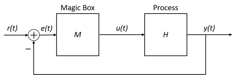
Fig. 11 A feedback control system#
So far, we have naively been using raw sensor data as our \(y(t)\) measurement. More specifically, we’ve been using the range reported by the drone’s downward facing IR sensor as the “ground truth” measurement of altitude.
However, there are a few problems with this:
In the real world, actual sensor hardware is not perfect – there’s noise in sensor readings. For example, a $10 TOF sensor might report a range of 0.3m in altitude, when in reality the drone is at 0.25m. While a more expensive sensor would be less susceptible to noise, it would still not be perfect.
The sensor readings may not really represent the behavior we wish to control. For example, it might seem like a downward facing TOF would be a good representation of a drone’s altitude, but suppose the drone rolls a non-trivial amount \(\theta or flies over a reflective surface\) (See Fig. 12).
No one sensor may be enough to measure the \(y(t)\) we really care about. For example, two 2D cameras would be needed to measure depth for a depth controller.
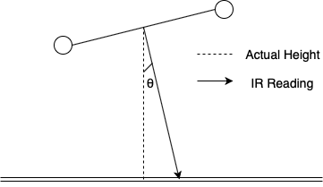
Fig. 12 An example of inaccurate sensor reading#
These problems imply that we need a higher-level abstraction for our \(y(t)\), namely one that accounts for: noise, robot motion, and sensor data. Let \(\mathbf{x}_{t}\) be such an abstraction called state. For example, \(\mathbf{x}_{t} = [\textit{altitude at time t}]\) for the purposes of altitude control. To account for noise, we should consider the distribution of possible states at time t:
Furthermore, let \(\mathbf{z}_{1:t}\) represent readings from all sensors from time 1 to \(t\). Likewise, let \(\mathbf{u}_{1:t}\) represent all robot motions from time 1 to \(t\). Then we can account for robot motion and sensor data on our distribution via conditioning:
Let this distribution be known as \(bel(\mathbf{x}_{t})\), i.e. the belief of the state of our dynamic system at time \(t\). Suppose, hypothetically, that we knew the distribution \(bel(\mathbf{x}_{t})\) (though we haven’t discussed how to determine it yet). Then we could change \(y(t)\) in our control system from a naïve sensor reading to:
For a specific \(x_{t}\) in the state vector \(\mathbf{x}_{t}\) (e.g. the altitude element in \(\mathbf{x}_{t}\)). Consequently, this would make \(e(t)\) in a feedback control system:
Understand \(bel(\mathbf{x}_{t})\)#
Although \(bel(\mathbf{x}_{t})\) seems to solve all our problems, it is unclear how to determine it explicitly. One way to do so is to decompose it into quantities that are easier to determine. Furthermore, it may prove helpful to make a few reasonable assumptions that will simplify the decomposition. In this vain, consider instead the distribution:
which is called the measurement model. It is probably reasonable to assume that knowing the state at time \(t\) is enough to determine the distribution of our sensor data; knowing all previous states, motions, and sensor data probably won’t add any new info. So our first simplification is a Markov assumption about the measurement model:
Likewise, consider the distribution:
Which is called the motion model. It is probably reasonable to assume that the state at time t only depends on the previous state and the motion that happened since. So another simplification is the Markov assumption about the motion model:
Why did we bother with an aside about these distributions and assumptions? Because they allow us to decompose \(bel(\mathbf{x}_{t})\) as follows:
where
and \(\eta\) is a constant. This decomposition gives rise to the Bayes Filter algorithm (see sections below). So effectively, it has reduced the challenge of determining the unknown (and difficult to figure out) distribution \(P(\mathbf{x}_{t}|\mathbf{z}_{1:t}, \mathbf{u}_{1:t})\) into figuring out the distributions \(P(z_{t}|x_{t})\) and \(P(\mathbf{x}_{t}|\mathbf{x}_{t-1}, \mathbf{u}_{t})\), i.e. measurement and motion models respectively.
Fortunately, these distributions are easier to figure out than \(bel(\mathbf{x}_{t})\); we can either determine these distributions experimentally for a robot or we can make assumptions about the PDF class of these functions (see next section).
Bayes Filter Extension#
So far we’ve reduced the challenge of determining \(bel(\mathbf{x}_{t})\) explicitly to instead determining \(P(z_{t}|x_{t})\) and \(P(\mathbf{x}_{t}|\mathbf{x}_{t-1}, \mathbf{u}_{t})\). One way to “determine” these is to purposefully assume they are distributions from well known parameterized PDF classes. A popular choice would the class of Gaussians, i.e. \(\mathcal{N}(\mu,\,\sigma^{2})\,\), which is a class parameterized by mean \(\mu\) and variance \(\sigma^{2}\); each \((\mu, \sigma^{2})\) pair gives a different-shaped bell curve.
So we assume:
where \(f\) and \(g\) are linear functions, \(k_{1}\) and \(k_{2}\) are some pre-determined variances. Together, these assumptions lead to \(bel(\mathbf{x}_{t})\) being a Gaussian as well:
Which gives rise to the Kalman Filter algorithm (see sections below). Note that the KF algorithm has the same form as the Baye’s Filter algorithm (since the base derivation is the same), but the KF algorithm only needs to find \(\mu_{t}\) and \(\sigma^{2}_{t}\) at each time step \(t\).
Practically, using a Kalman Filter means providing linear functions \(f\) and \(g\) as input. What are \(f\) and \(g\)?
\(f\) is a function that captures the motion dynamics of a system. Simply put, \(f\) can be thought of as calculating the “predicted” \(\mathbf{x}_{t}\) after motion. For example, suppose we have a drone that moves only horizontally. Let state \(\mathbf{x}_{t}\) be the horizontal position \(x\_pos\) at time t, \(\mathbf{u}_{t}\) be the horizontal velocity \(v_{t}\) (i.e. the control signal we send the drone), and \(\mathbf{\widehat{x}}_{t}\) is the predicted state due to motion. Then:
\(g\) is a function that transforms the state into something that can be compared to the sensor data \(\mathbf{z}_{t}\). Simply put, \(g(\mathbf{x}_{t})=\mathbf{\widehat{z}}_{t}\), i.e. a “predicted” sensor reading based on the current state. For example: suppose a drone is rolled by \(\theta\), \(\mathbf{z}_{t} = [r]\) for a range \(r\) reported by an IR sensor, and \(\mathbf{x}_{t}\) is \([d, \theta]\) for an altitude of \(d\) and roll of \(\theta\):
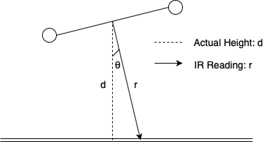
Fig. 13 An example of ir measurement calculation#
Then a non-linear \(g\) woould be:
A key requirement of the Kalman Filter algorithm is that \(f\) and \(g\) need to be linear functions. This is necessary in order for the various Gaussians to multiply such that \(bel(\mathbf{x}_{t})\) is still a Gaussian. Under the assumption of linearity, the Kalman Filter is provably optimal.
However, most systems which have non-linearities. For example, the drone’s update function involves nonlinear trigonometric functions like sin and cosine. Many people use the Extended Kalman Filter(EKF) algorithm instead. The EKF handles non-linear functions by basically doing a first-order Taylor expansion (to create a linear approximation) on \(f\) and \(g\), then passing them to the Kalman Filter algorithm. To perform this approximation, the Jacobian matrix of \(f\) and \(g\) must be computed (e.g., the deriviative with respect to every input variable.) This Jacobian matrix must be derived and then implemented in code, an non-trivial effort.
Fortunately, another alternative is the Unscented Kalman Filter(UKF) algorithm, which is a sampling-based variant of the Kalman Filter. Like the EKF, the UKF can handle non-linear \(f\) and \(g\). The UKF is not only simpler to implement than the EKF, it also performs better, although it is not provably optimal.
Background before UKF#
Before we dive into the UKF, there are some foundations that we should build up:
Estimating by averaging
The Bayes Filter
Gaussians
The Kalman Filter
The basis for the Kalman Filter lies in probability; as such, if you want to better understand some of these probabilistic algorithms, you may find it helpful to brush up on probability. A useful reference on probability and uncertainty is [Jay03].
Since the UKF is an adaptation of the standard Kalman Filter, a lot of our discussion will apply to Kalman Filters in general.
Estimating by Averaging#
Imagine a simple one-dimensional system in which your drone moves along the \(z\)-axis by adjusting its thrust. The drone has a downward-pointing infrared (IR) range sensor that offers you a sense of the drone’s altitude, albeit with noise, as the sensor is not perfect. You are aware of this noise and want to eliminate it: after all, you know by empirical observation that your drone does not oscillate as much as the noisy IR range readings suggest, and that the average value of a lot of IR readings gets you a close estimate of the actual height. What can you do? A simple solution is to average recent range readings so as to average out the noise and smooth your estimate. One way to implement this is with a moving average that computes a weighted sum of the previous average estimate and the newest measurement.
where \(\mathbf{\hat x}_t\) is the weighted average of the drone’s state (here, just its height) at time \(t\) computed by weighting the previous average \(\mathbf{\hat x}_{t - \Delta t}\) by a scalar \(\alpha\) between \(0\) and \(1\) and the new measurement \(\mathbf{z}_t\) (here, just the raw IR reading) by \((1 - \alpha)\). A higher \(\alpha\) will result in a smoother estimate that gives more importance to the previous average than the new measurement; as such, a smoother estimate results in increased latency.
This approach works for many applications, but for our drone, we want to be able to know right away when it makes a sudden movement. Averaging the newest sensor reading with past readings suffers from latency, as it takes time for the moving average to approach the new reading. Ideally we would be able to cut through the noise of the IR sensor and experience no latency. We will strive for this kind of state estimation.
As a related thought experiment, imagine that you do not have control of the drone but are merely observing it from an outsider’s perspective. In this scenario, there is one crucial bit of information that we lack: the control input that drives the drone. If we are controlling the drone, then presumably we are the ones sending it commands to, for example, accelerate up or down. This bit of information is useful (but not necessary) for the Bayes and Kalman Filters, as we will discuss shortly. Without this information, however, employing a moving average to estimate altitude is not a bad approach.
The Bayes Filter#
To be able to get noise-reduced estimates with less latency than a via an averaging scheme, we can look to a probabilistic method known as the Bayes Filter, which forms the basis for Kalman filtering and a number of other probabilistic robotics algorithms. The idea with a Bayes Filter is to employ Bayes’ Theorem and the corresponding idea of conditional probability to form probability distributions representing our belief in the robot’s state (in our one-dimensional example, its altitude), given additional information such as the robot’s previous state, a control input, and the robot’s predicted state.
Say we know the drone’s state \(\mathbf{x}_{t-\Delta t}\) at the previous time step as well as the most recent control input \(\mathbf{u}_t\), which, for example, could be a command to the motors to increase thrust. Then, we would like to find the probability of the drone being at a new state \(\mathbf{x}_t\) given the previous state and the control input. We can express this with conditional probability as:
This expression represents a prediction of the drone’s state, also termed the prior, as it is our estimate of the drone’s state before incorporating a measurement. Next, when we receive a measurement from our range sensor, we can perform an update, which looks at the measurement and the prior to form a posterior state estimate. In this step, we consider the probability of observing the measurement \(\mathbf{z}_t\) given the state estimate \(\mathbf{x}_t\):
By Bayes’ Theorem, we can then derive an equation for the probability of the drone being in its current state given information from the measurement:
After a little more manipulation and combining of the predict and update steps, we can arrive at the Bayes Filter algorithm [TBF05]:
\(\hspace{5mm} \text{Bayes\_Filter}(bel(\mathbf{x}_{t-\Delta t}), \mathbf{u}_t, \mathbf{z}_t):\)
\(\hspace{10mm} \text{for all } \mathbf{x}_t \text{ do}:\)
\(\hspace{15mm} \bar{bel}(\mathbf{x}_t) = \int p(\mathbf{x}_t \mid \mathbf{u}_t, \mathbf{x}_{t-\Delta t})bel(\mathbf{x}_{t-\Delta t})\mathrm{d}\mathbf{x}\)
\(\hspace{15mm} bel(\mathbf{x}_t) = \eta p(\mathbf{z}_t \mid \mathbf{x}_t)\bar{bel}(\mathbf{x}_t)\)
\(\hspace{10mm} \text{endfor}\)
\(\hspace{10mm} \text{return } bel(\mathbf{x}_t)\)
The filter calculates the probability of the robot being in each possible state \(\mathbf{x}_t\) (hence the \(\text{for}\) loop). The prediction is represented as \(\bar{bel}(\mathbf{x}_t)\) and embodies the prior belief of the robot’s state after undergoing some motion, before incorporating our most recent sensor measurement. In the measurement update step, we compute the posterior \(bel(\mathbf{x}_t)\). The normalizer \(\eta\) is equal to the reciprocal of \(p(\mathbf{z}_t)\); alternatively, it can be computed by summing up \(p(\mathbf{z}_t \mid \mathbf{x}_t)\bar{bel}(\mathbf{x}_t)\) over all states \(\mathbf{x}_t\). This normalization ensures that the new belief \(bel(\mathbf{x}_t)\) integrates to 1.
Gaussians#
Bayes Filter is a useful concept, but often it is too difficult to compute the beliefs, particularly with potentially infinite state spaces. We want to then find a useful way to represent these probability distributions in a manner that accurately represents the real world while also making computation feasible. To do this, we exploit Gaussian functions.
We can represent the beliefs as Gaussian functions with a mean and a covariance matrix. Why? The state variables and measurements are random variables in that they can take on values in their respective sample spaces of all possible states and measurements. By the Central Limit Theorem, these random variables will be distributed normally (i.e., will form a Gaussian probability distribution) when you take a lot of samples. The Gaussian assumption is a strong one: think of a sensor whose reading fluctuates due to noise. If you take a lot of readings, most of the values should generally be concentrated in the center (the mean), with more distant readings occurring less frequently.
We use Gaussians because they are a good representation of how noise is distributed and because of their favorable mathematical properties. For one, Gaussians can be described by a mean and a covariance, which require less bookkeeping. Furthermore, Gaussian probability density functions added together result in another Gaussian, and products of two Gaussians (i.e., a joint probability distribution of two Gaussian distributions) are proportional to Gaussians [Jr18], which makes for less computation than if we were to use many samples from an arbitrary probability distribution. The consequence of these properties is that we can pass a Gaussian through a linear function and recover a Gaussian on the other side. Similarly, we can compute Bayes’ Theorem with Gaussians as the probability distributions, and we find that the resulting probability distribution will be Gaussian [Jr18].
In the Bayes Filter, we talked about the predict and update steps. The prediction uses a state transition function, also known as a motion model, to propagate the state estimate (which we can represent as a Gaussian) forward in time to the next time step. If this function is linear, then the prior state estimate will also be Gaussian. Similarly, in the measurement update, we compute a new distribution using a measurement function to be able to compare the measurement and the state. If this function is linear, then we can get a Gaussian distribution for the resulting belief. We will elaborate on this constraint of linearity when we discuss the usefulness of the Unscented Kalman Filter, but for now you should be comfortable with the idea that using Gaussians to represent the drone’s belief in its state is a helpful and important modeling assumption.
Multivariate Gaussians#
Most of the time when we implement a Kalman Filter, we track more than one state variable in the state vector (we will go over what these terms mean and some intuition for why we do this in the next section). We also often receive more than one control and measurement input. What this means is that, as you may have noticed in the above equations which contain boldface vectors, we want to represent state estimates in more than one dimension in state space. As a result, our Gaussian representations of these state estimates will be multivariate. We won’t go into much detail about this notion except to point out, for example, that tracking multiple state variables with a multivariate Gaussian (represented as a vector of means and a covariance matrix) allows us to think about how different state variables are correlated. Again, we will cover this in greater detail as we talk about Kalman Filters in the following section—now you know, however, that there is motivation for using multi-dimensional Gaussians. If you want to learn more about this topic, we recommend [Labbe’s textbook][Jr18], which also contains helpful graphics to understand what is going on with these Gaussians intuitively.
The Kalman Filter#
High-Level Description of the Kalman Filter Algorithm#
Recall from the Bayes Filter the procedure of carrying out predictions and measurement updates. The Kalman Filter, an extension of Bayes Filter with Gaussian assumptions on the belief distributions, aims to fuse measurement readings with predicted states. For example, if we know (with some degree of uncertainty) that the drone is moving upward, then this knowledge can inform us about the drone’s position at the next time step. We can form a prediction of the drone’s state at the next time step given the drone’s current state and any control inputs that we give the drone. Then, at the next time step when we receive a new measurement, we can perform an update of our state estimate. In this update step, we look at the difference between the new measurement and the predicted state. This difference is known as the residual. Our new state estimate (referred to in literature as the posterior) lies somewhere between the predicted state, or prior, and the measurement; the scaling factor that accomplishes this is known as the Kalman gain [Jr18]. Fig. 14 depicts this process of prediction and measurement update.
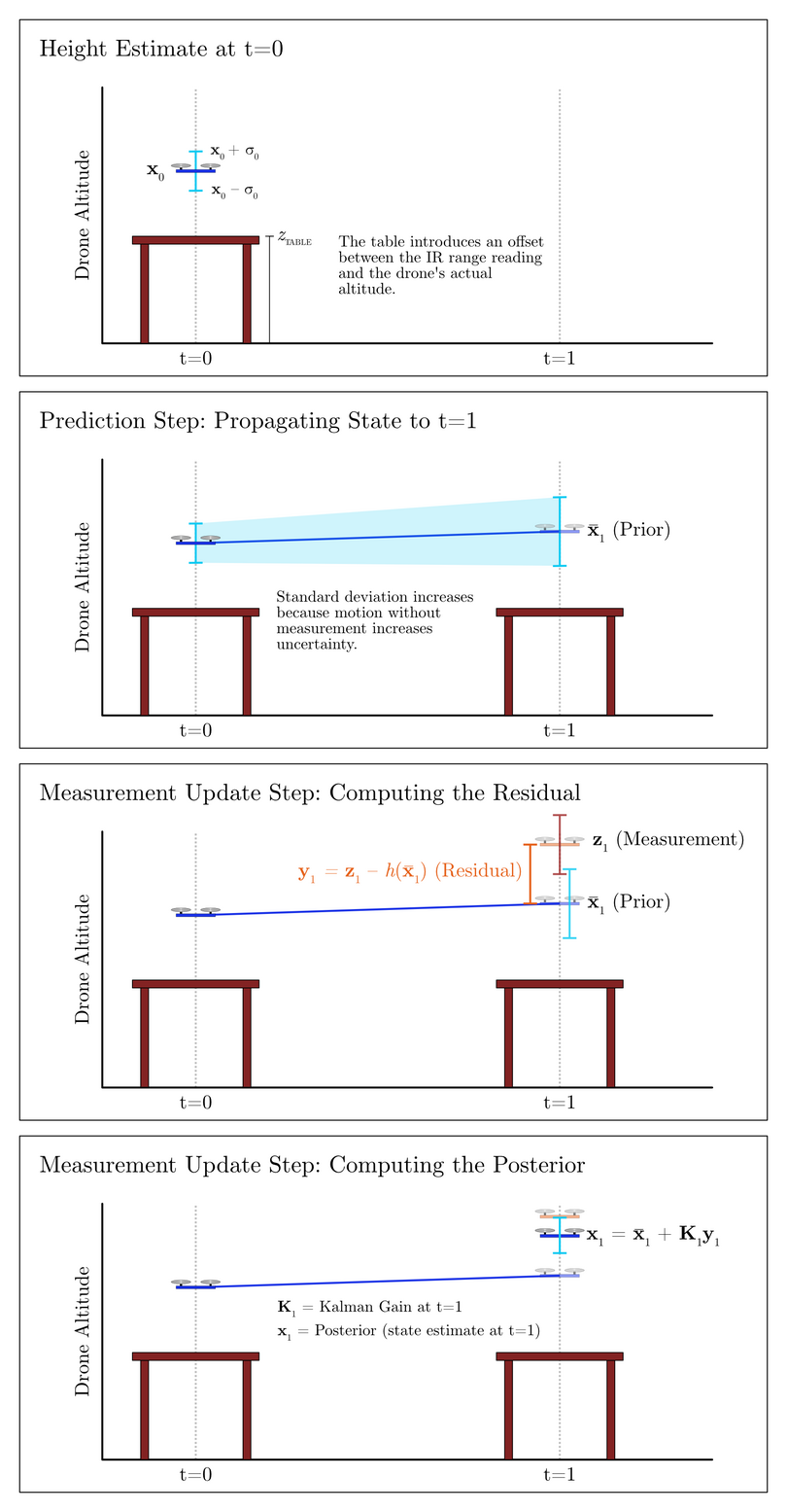
Fig. 14 Predict-Update Cycle for a Kalman Filter Tracking a Drone’s Motion in One Dimension#
State Vector and Covariance Matrix#
The KF accomplishes its state estimate by tracking certain state variables in a state vector, such as position and velocity along an axis, and the covariance matrix corresponding to the state vector. In the first part of this project, your UKF’s state vector will track the drone’s position and velocity along the \(z\)-axis and will look like:
where \(z\) and \(\dot z\) are the position and velocity of the drone along the \(z\)-axis, respectively. Fig. 14 depicts a contrived example in which the drone is hovering above a table. We will describe why we show this contrived example shortly when we discuss the measurement function, but for now, you should focus on the fact that we want to know the drone’s position along the \(z\)-axis (where the ground is 0 meters) and its velocity.
Why did we decide to track not only position but also velocity? What if we were only interested in the drone’s position along the \(z\)-axis? Well, while in some cases we might only be immediately interested in, say, knowing the robot’s position, the addition of \(\dot z\) is also important. \(\dot z\) is known as a hidden variable: we do not have a sensor that allows us to measure this quantity directly. That said, keeping track of this variable allows us to form better estimates about \(z\). Why? Since position and velocity are correlated quantities, information about one quantity can inform the other. If the drone has a high positive velocity, for instance, we can be fairly confident that its position at the next time step will be somewhere in the positive direction relative to its previous position. The covariances between position and velocity allow for a reasonable estimate of velocity to be formed—as does any information about acceleration, for example. Chapter 5.7 of Labbe’s textbook [Jr18] describes the importance of this correlation between state variables such as position and velocity. In addition, as you will see when we discuss the state transition model of a Kalman Filter, the control input impacts the prior state estimate. In this particularly instance, the control input is a linear acceleration value, which can be integrated to provide information about velocity.
The state vector tracks the mean \(\mu_t\) of each state variable, which—as we noted in the section on Gaussians—we assume is normally distributed about \(\mu_t\). To characterize the uncertainty in this state estimate, we use an \(n \times n\) covariance matrix where \(n\) is the size of the state vector. For this state vector, then, we define the covariance matrix as:
where \(\sigma^2_z = \text{Var}\left( z \right)\), for example, denotes the variance in the position estimates and \(\sigma_{\dot z,z} = \sigma_{z,\dot z} = \text{Cov}\left( z, \dot z \right)\) denotes the covariance between the position and velocity estimates. As mentioned above, position and velocity are typically positively correlated, as a positive velocity indicates that the drone will likely be at a more positive position at the next time step.
The first frame of Fig. 14 illustrates a state estimate and the standard deviation of that height estimate.
State Transition Model for the Prediction Step#
The part of the KF that computes a predicted state \(\mathbf{\bar x}_t\) is known as the state transition function. The prediction step of the UKF uses the state transition function to propagate the current state at time \(t-\Delta t\) to a prediction of the state at the next time step, at time \(t\). In standard Kalman Filter literature for linear systems, this transition function can be expressed with two matrices: a state transition matrix \(\mathbf{A}_t\) and a control function \(\mathbf{B}_t\) that, when multiplied with the current state vector \(\mathbf{x}_{t-\Delta t}\) and with the control input vector \(\mathbf{u}_t\), respectively, sum together to output the prediction of the next state.
We give \(\mathbf{A}_t\) and \(\mathbf{B}_t\) each a subscript \(t\) to indicate that these matrices can vary with time. Often, these matrices will include one or more \(\Delta t\) terms in order to properly propagate the state estimate forward in time by that amount. If our control input, for example, comes in at a varying frequency, then the time step \(\Delta t\) will change.
More generally, in nonlinear systems—where the UKF is useful, which we will describe later—a single transition function \(g(\mathbf{x}_{t-\Delta t}, \mathbf{u}_t, \Delta t)\) can express the prediction of what the next state will be given the current state estimate \(\mathbf{x}_{t-\Delta t}\), the control input \(\mathbf{u}_t\), and the time step \(\Delta t\) [TellexBrownLupashin18]. For robotic systems such as the Duckiedrone, the state transition function often involves using kinematic equations to form numerical approximations of the robot’s motion in space.
The control input that you will use for this project is the linear acceleration along the \(z\)-axis \(\ddot z\) being output by the IMU. While the distinction between this control input and other measurements might seem vague, we can think of these acceleration values as being commands that we set when we control the drone. Indeed, since we control the drone’s throttle and thus the downward force of the propellers, we do control the drone’s acceleration by Newton’s Second Law of Motion:
That said, even though in practice people do successfully use IMU accelerations as control inputs, research [EE15] indicates that in certain cases it may be better to use IMU data in the measurement update step; this is an example of a design decision whose performance may depend on the system you are modeling. We choose to use the IMU’s acceleration as the control input \(\mathbf{u}_t\):
Expressing Newton’s Second Law in terms of our control input, we have:
which denotes that the net force \(\mathbf{F}\) acting on the drone is equal to its mass \(m\) (assumed to be constant) multiplied by the acceleration \(\ddot z\) in the \(\hat{z}\) direction (i.e., along the \(z\)-axis).
The second frame of Fig. 14 shows the result of the state transition function: the drone’s state estimate has been propagated forward in time, and in doing so, the uncertainty in its state has increased, since its motion model has some degree of uncertainty and the new measurement has not yet been incorporated.
Measurement Function#
After the prediction step of the KF comes the measurement update step. When the drone gets a new measurement from one of its sensors, it should compute a new state estimate based on the prediction and the measurement. In the \(z\)-axis motion model for the first part of this project, the sensor we consider is the infrared (IR) range sensor. We assume that the drone has no roll and pitch, which means that the IR reading directly corresponds to the drone’s altitude. The measurement vector, then, is defined as:
where \(r\) is the IR range reading.
In our contrived example shown in Fig. 14, however, the IR range reading does not directly correspond to the drone’s altitude: there is an offset due to the height of the table \(z_{\text{TABLE}}\).
As depicted in the third frame of Fig. 14, part of the measurement update step is the computation of the residual \(\mathbf{y}_t\). This value is the difference between the measurement and the predicted state. However, the measurement value lives in measurement space, while the predicted state lives in state space. For your drone’s particular 1D example (without the table beneath the drone), the measurement and the position estimate represent the same quantity; however, in more complicated systems such as the later part of this project in which you will be implementing a UKF to track multiple spatial dimensions, you will find that the correspondence between measurement and state may require trigonometry. Also, since the sensor measurement often only provides information pertaining to part of the state vector, we cannot always transform a measurement into state space. Chapter 6.6.1 of Labbe’s textbook [Jr18] describes the distinction between measurement space and state space.
Consequently, we must define a measurement function \(h(\mathbf{\bar x}_t)\) that transforms the prior state estimate into measurement space. (For the linear Kalman Filter, this measurement function can be expressed as a matrix \(\mathbf{H}_t\) that gets multiplied with \(\mathbf{\bar x}_t\).) As an example, our diagrammed scenario with the table requires the measurement function to account for the height offset. In particular, \(h(\mathbf{\bar x}_t)\) would return a \(1 \times 1\) matrix whose singular element is the measurement you would expect to get with the drone positioned at a height given by the \(z\) value in the prior \(\mathbf{\bar x}_{t,z}\):
This transformation allows us to compute the residual in measurement space with the following equation:
Once the residual is computed, the posterior state estimate is computed via the following equation:
where \(\mathbf{K}_t\) is the Kalman gain that scales how much we “trust” the measurement versus the prediction. Once this measurement-updated state estimate \(\mathbf{x}_t\) is calculated, the filter continues onto the next predict-update cycle.
The fourth frame of Fig. 14 illustrates this fusion of prediction and measurement in which a point along the residual is selected for the new state estimate by the Kalman gain. The Kalman gain is determined mathematically by taking into account the covariance matrices of the motion model and of the measurement vector. While we do not expect you to know exactly how to compute the Kalman gain, intuitively it is representative of a ratio between the uncertainty in the prior and the uncertainty in the newly measured value.
At a high level, that’s the Kalman Filter algorithm! Below is the general linear Kalman Filter algorithm [TellexBrownLupashin18] [TBF05] [Jr18] written out in pseudocode. We include \(\Delta t\) as an argument to the \(\text{predict}()\) function since it so often is used there. We use boldface vectors and matrices to describe this algorithm for the more general multivariate case in which we are tracking more than one state variable, we have more than one measurement variable, et cetera. We also have not yet introduced you to the \(\mathbf{Q}_t\) and \(\mathbf{R}_t\) matrices; you will learn about them later in this project when you implement your first filter. Also, we did not previously mention some of the equations written out in this algorithm (e.g., the computation of the Kalman gain); fret not, however, as you are not responsible for understanding all of the mathematical details. Nonetheless, we give you this algorithm for reference and for completeness. As an exercise, you might also find it helpful to compare the KF algorithm to the Bayes Filter algorithm written above.
\(\hspace{5mm} \textbf{function}\text{ predict}( \mathbf{x}_{t-\Delta t},
\mathbf{P}_{t-\Delta t}, \mathbf{u}_t, \Delta t )\)
\(\hspace{10mm} \texttt{// Compute predicted mean}\)
\(\hspace{10mm} \mathbf{\bar x}_t = \mathbf{A}_t \mathbf{x}_{t-\Delta t} +
\mathbf{B}_t \mathbf{u}_t\)
\(\hspace{10mm} \texttt{// Compute predicted covariance matrix}\)
\(\hspace{10mm} \mathbf{\bar P}_t = \mathbf{A}_t \mathbf{P}_{t-\Delta t} \mathbf{A}_t^\mathsf{T} +
\mathbf{Q}_t\)
\(\hspace{10mm} \text{return } \mathbf{\bar x}_t, \mathbf{\bar P}_t\)
\(\hspace{5mm} \textbf{function}\text{ update}(\mathbf{\bar x}_t,
\mathbf{\bar P}_t, \mathbf{z}_t)\)
\(\hspace{10mm} \texttt{Compute the residual in measurement space}\)
\(\hspace{10mm} \mathbf{y}_t = \mathbf{z}_t - \mathbf{H}_t \mathbf{\bar x}_t\)
\(\hspace{10mm} \texttt{Compute the Kalman gain}\)
\(\hspace{10mm} \mathbf{K}_t = \mathbf{\bar P}_t \mathbf{H}_t^\mathsf{T} \left(
\mathbf{H}_t \mathbf{\bar P}_t \mathbf{H}_t^\mathsf{T} + \mathbf{R}_t \right)^{-1}\)
\(\hspace{10mm} \texttt{Compute the mean of the posterior state estimate}\)
\(\hspace{10mm} \mathbf{x}_t = \mathbf{\bar x}_t + \mathbf{K}_t\mathbf{y}_t\)
\(\hspace{10mm} \texttt{Compute the covariance of the posterior state estimate}\)
\(\hspace{10mm} \mathbf{P}_t = \left( \mathbf{I} - \mathbf{K}_t \mathbf{H}_t \right) \mathbf{\bar P}_t\)
\(\hspace{10mm} \text{return } \mathbf{x}_t, \mathbf{P}_t\)
\(\hspace{5mm} \textbf{function}\text{ kalman\_filter}( \mathbf{x}_{t-\Delta t},\mathbf{P}_{t-\Delta t} )\)
\(\hspace{10mm} \mathbf{u}_t = \text{get\_control\_input}()\)
\(\hspace{10mm} \Delta t = \text{compute\_time\_step}()\)
\(\hspace{10mm} \mathbf{\bar x}_t, \mathbf{\bar P}_t = \text{predict}(\mathbf{x}_{t-\Delta t}, \mathbf{P}_{t-\Delta t}, \mathbf{u}_t, \Delta t )\)
\(\hspace{10mm} \mathbf{z}_t = \text{get\_sensor\_data}()\)
\(\hspace{10mm} \mathbf{x}_t, \mathbf{P}_t = \text{update}(\mathbf{\bar x}_t,\mathbf{\bar P}_t, \mathbf{z}_t)\)
\(\hspace{10mm} \text{return } \mathbf{x}_t, \mathbf{P}_t\)
- EE15
A. T. Erdem and A. Ö. Ercan. Fusing inertial sensor data in an extended kalman filter for 3d camera tracking. IEEE Transactions on Image Processing, 24(2):538–548, Feb 2015. doi:10.1109/TIP.2014.2380176.
- Jay03
Edwin T Jaynes. Probability theory: The logic of science. Cambridge university press, 2003.
- Jr18(1,2,3,4,5,6,7)
Roger R Labbe Jr. Kalman and bayesian filters in python. Published as a Jupyter Notebook hosted on GitHub at https://github.com/rlabbe/Kalman-and-Bayesian-Filters-in-Python and in PDF form at https://drive.google.com/file/d/0By_SW19c1BfhSVFzNHc0SjduNzg/view?usp=sharing (accessed August 29, 2018), May 2018.
- TBF05(1,2)
Sebastian Thrun, Wolfram Burgard, and Dieter Fox. Probabilistic Robotics (Intelligent Robotics and Autonomous Agents). The MIT Press, 2005. ISBN 0262201623.
- TellexBrownLupashin18(1,2)
S. Tellex, A. Brown, and S. Lupashin. Estimation for Quadrotors. ArXiv e-prints, August 2018. arXiv:1809.00037.