Demo - Lane Following
Contents
Demo - Lane Following#
This chapter describes the Lane Following (LF) demo (demonstration) for Duckiebots.
What you will need
A calibrated Duckiebot: Operations - Calibrations
Completed Camera Calibration.
Completed Wheel Calibration.
A Duckietown, as defined in The Duckietown Operation Manual.
Good lighting (ideally white diffused light). This demo relies on images from the camera and color detections. Therefore, avoid colored lights, reflections or other conditions that may confuse or blind the on-board image sensor.
What you will get
A Duckiebot driving autonomously in a Duckietown without obstacles, intersections or other Duckiebots.
Introduction to lane following#
Setup#
To set up the demo:
Place your Duckiebot in a lane such that it will drive on the right-hand side of the road, making sure that it sees the lane lines.
Stop any running containers on your Duckiebot that use its camera or control its motors.
Start#
To run the demo on your Duckiebot in Debug mode, run:
dts duckiebot demo --demo_name lane-following --duckiebot_name DUCKIEBOT_NAME --debug
Note
Your Duckiebot’s LEDs should turn green.
Attention
To quickly stop your Duckiebot, press E (Emergency Stop).
To start lane following:
Open a new terminal.
Run
dts duckiebot keyboard_control DUCKIEBOT_NAME.With the
Keyboard Controlwindow in focus, press F (Autopilot).
Note
Your Duckiebot’s front and back LEDs should turn white and red, respectively, and it should start following the lane it is in.
Note
If intersections and/or red lines are present in the layout, they will be neglected and your Duckiebot will drive across them as if it were in a normal lane.
Note
If this demo does not work as expected, follow Debugging and parameter tuning or Troubleshooting.
Stop#
To stop lane following:
Click the
Keyboard Controlwindow if it is not in focus.Press F (
Autopilot).
Note
Your Duckiebot’s LEDs should turn green and it should stop following the lane it is in.
To stop the demo:
Select the terminal from which the demo was run.
Press Ctrl+C.
Visualize#
To see what your Duckiebot sees and other visualizations related to the demo:
Run
dts duckiebot image_viewer DUCKIEBOT_NAME.Select a topic from the drop-down menu.
How it works#
The Lane Following demo consists of the following processing steps:
Image capture (an image is captured from your Duckiebot’s camera).
Line detection (colored line segments in the captured image are detected).
Ground projection (based on the camera’s known intrinsic and extrinsic parameters, the detected line segments are projected onto the ground plane).
Lane estimation (the ground projected line segments and motion of your Duckiebot, which can be estimated with the help of its wheel encoders, are used to produce an estimate of your Duckiebot’s lane pose).
Control (based on the lane pose estimate, a PID controller sends control signals to adjust your Duckiebot’s heading).
Actuation (the control signals are applied to your Duckiebot’s motors).
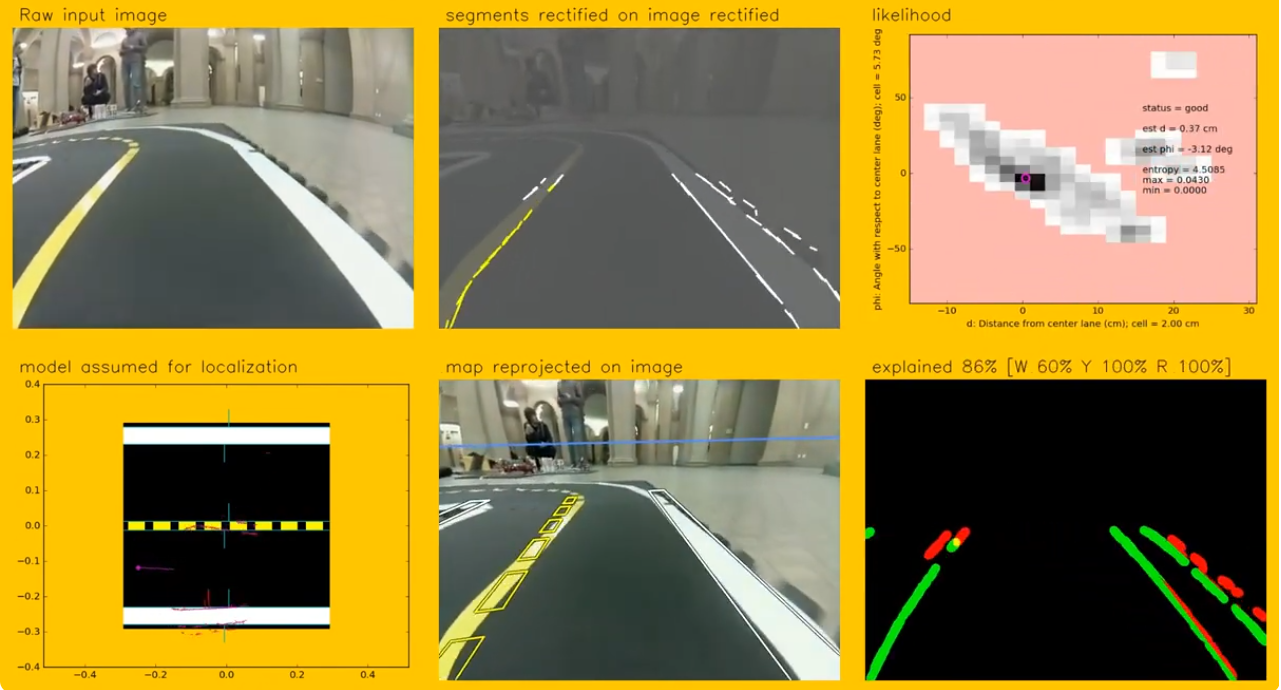
Fig. 46 Lane following processing flow, from input image to belief.#
Line detection#
Line detection involves extracting line segments from an image, focusing on specific colors that correspond to lane markers (white, yellow and red). This process combines multiple stages color filtering, edge detection and line segment extraction, and is designed to efficiently detect lane lines in Duckietowns.
Preprocessing#
Images are preprocessed for more effective feature extraction. For example, blurring the image using a Gaussian blur, converting the image to the HSV (Hue, Saturation and Value) color space. HSV is preferred over RGB (Red, Green and Blue) for color segmentation, as it separates chromatic content (hue) from intensity (value), making it easier to isolate specific colors. Then, a color range filter is applied to segment regions corresponding to marker colors (e.g., white, yellow and red). This operation results in a binary mask, highlighting only the regions of interest.
Edge detection#
To identify edges, filtered images are passed through the Canny edge detection algorithm, which consists of a gradient calculation, non-maximum suppression and hysteresis thresholding.
Gradient calculation: The image gradient is computed using the Sobel operator, which highlights areas of rapid intensity change (\(G = \sqrt{G_x^2 + G_y^2}\), where \(G_x = \frac{\partial I}{\partial x}\) and \(G_y = \frac{\partial I}{\partial y}\)).
Non-maximum suppression: Edges are thinned out by suppressing the pixels that are not part of the edge contours.
Hysteresis thresholding: Two thresholds (\(T_{low}\) and \(T_{high}\)) are applied to classify edges as strong, weak or irrelevant. Edges stronger than \(T_{high}\) are retained and weak edges connected to strong ones are kept.
Line segment extraction#
The detected edges are analyzed to extract line segments using the Hough line transform. This method identifies lines in the image by voting in the parameter space:
Each edge point \((x, y)\) contributes a vote for all possible lines passing through it, represented in polar coordinates as \(\rho = x\cos(\theta) + y\sin(\theta), \), where \(\rho\) is the distance from the origin to the line and \(\theta\) is the angle of the line normal.
A threshold on the accumulator ensures that only lines with sufficient votes are retained.
While these are the main components involved, there are additional post processing steps that can be done, as well as the tuning of some hyperparameters to optimize performance.
Ground projection#
Detected line segments are transformed from the camera’s image plane to the ground plane using the homography matrix. This transformation allows your Duckiebot to localize itself and navigate its environment effectively.
Homography and calibration#
The homography matrix is obtained through an extrinsic calibration procedure, which establishes the spatial relationship between the camera and the ground plane. The transformation is represented as \(P_w = H P_c\), where \(P_w = (x, y, 1)\) and \(P_c = (u, v, 1)\). \((u, v)\) are the pixel coordinates in the image, \((x, y)\) are the corresponding coordinates in the ground plane, and \(H\) is the homography matrix.
Input and processing#
Line segments are first rectified using the intrinsic parameters to correct for distortions, ensuring accurate mappings.
Ouput#
Projected line segments are represented in the ground plane, providing a useful representation for downstream tasks such as lane localization and control. Additionally, debug images showing rectified and projected views are published for verification.
Lane estimation#
The histogram filter is used to estimate your Duckiebot’s lane pose (\(d\), \(\phi\)), where \(d\) is its lateral deviation relative to the lane’s center and \(\phi\) is its angular deviation relative to the lane’s orientation. This probabilistic approach provides a robust way to localize your Duckiebot using noisy sensor data while accounting for uncertainty. This filter maintains a discrete grid over the deviation values, where each grid cell represents a possible state of your Duckiebot.
This filter is recursive, meaning that it iterates between predicting the next state of your Duckiebot, using its known kinematic model and the data from its wheel encoders, and updating, based on the ground projected lane segments.
Prediction step#
During the prediction step, the filter uses your Duckiebot’s estimated linear and angular velocities to update the histogram, predicting how its lane pose evolves over time. The state transition is modeled based on your Duckiebot’s kinematic model:
where \(v\) and \(\omega\) are the linear and angular velocities, respectively, and \(\Delta t\) is the time step. The predicted state probabilities are updated by shifting the histogram values accordingly.
Update step#
Detected line segments are projected onto the ground plane and matched to the expected lane geometry. For each segment:
The filter computes votes for possible \((d, \phi)\) values based on the segment’s position and orientation.
These votes are added to the corresponding bins in the histogram.
This process updates the belief distribution, increasing confidence in states consistent with the observations. The filter’s best estimate of the lane pose corresponds to the histogram cell with the highest value (maximum likelihood). This estimate is used to guide navigation.
Control#
With the state estimation provided by the histogram filter, a PID controller is used to send wheel commands to your Duckiebot. The PID controller calculates a control signal \(u_t\) based on the error \(e_t\) between the desired state (reference) and the estimated state:
where:
\(K_p\) is the proportional gain, addressing the current error.
\(K_i\) is the integral gain, correcting cumulative past errors.
\(K_d\) is the derivative gain, anticipating future errors based on the rate of change.
For lane following, the control inputs are the reference state \((d_{ref}, \phi_{ref})\) and the control outputs are a constant linear velocity \(v\) and a variable angular velocity \(\omega\) to correct for deviations. Using a linearized kinematic model and a constant forward velocity \(v\), the control law simplifies to:
where \(K_d\) and \(K_{\phi}\) are tuned proportional gains for lateral and angular errors, respectively.
Debugging and parameter tuning#
If the performance of your Duckiebot is inconsistent or poor, the following are some tips that you can use to debug the issue and tune the parameters of the various modules.
Build and run the code on your Duckiebot#
The code for the demo can be found in the dt-core repository.
To clone the dt-core repository, run:
git clone [email protected]:duckietown/dt-core.git --branch ente
To build the dt-core image on your Duckiebot, run the following command from the newly create dt-core directory:
dts devel build -H DUCKIEBOT_NAME
To run the demo on your Duckiebot, run the following command from the newly create dt-core directory:
dts devel run -H DUCKIEBOT_NAME -L lane-following
Tip
You can add a new DUCKIEBOT_NAME.yaml file to the config folder in any package in the dt-core repository and those parameters will be taken at startup in place of the ones specified in default.yaml
Tip
In most cases, you can modify the parameters using the utility rosparam set.
However, these values will not persist if you restart the demo until you change the actual values that are loaded from the config folder of the node.
Tuning the HSV thresholds#
To view the colormaps:
Run
dts duckiebot image_viewer DUCKIEBOT_NAME.Select the
NODE/line_detector_node/debug/maps/jpegtopic, whereNODEisDUCKIEBOT_NAME/node/image_relayer.
If the white or yellow regions of the image are not being well segmented, try tuning the color thresholds using a new dt-core/packages/line_detector/config/line_detector_node/DUCKIEBOT_NAME.yaml file.
The color thresholds are specified by the following thresholds, which are in HSV space as described above:
colors:
  RED:
    low_1: [0,140,100]
    high_1: [15,255,255]
    low_2: [165,140,100]
    high_2: [180,255,255]
  WHITE:
    low: [0,0,150]
    high: [180,100,255]
  YELLOW:
    low: [15,80,50]
    high: [45,255,255]
Note
You should not need to worry about the RED colors for now but the WHITE and YELLOW colors may need to be tuned depending on the type and amount of light in your environment.
Verifying the ground projections#
To view the lane pose and segment markers:
Run
dts duckiebot image_viewer DUCKIEBOT_NAME.Select the
NODE/ground_projection_node/debug/ground_projection_image/jpegtopic, whereNODEisDUCKIEBOT_NAME/node/image_relayer.
Note
You should see a top-down view of the lane in front of your Duckiebot.
If an error was incurred during the camera calibration procedure, it will be very apparent when looking at the ground projected segments.
Tuning the PID gains#
Tuning the PID gains is one of the most important aspects for the stability and performance of your Duckiebot, as:
The proportional gain (\(K_p\)) affects the magnitude of corrections. Too high a value leads to oscillations, while too low a value results in sluggish response.
The integral gain (\(K_i\)) addresses steady-state errors but can introduce instability if over tuned.
The derivative gain (\(K_d\)) smooths out the response by reducing overshoot but can amplify noise.
Troubleshooting#
Troubleshooting
SYMPTOM
The demo does not respond when pressing F.
RESOLUTION
Before trying to use the Keyboard Controller, make sure that it is active by selecting it’s window.
Troubleshooting
Troubleshooting
SYMPTOM
My Duckiebot does not drive nicely through intersections.
RESOLUTION
For this demo, there should not be any intersections in your Duckietown layout. Your Duckiebot will interpret intersections as “broken” lanes, perceiving less salient features, potentially compromising the state estimate.
Troubleshooting
SYMPTOM
My Duckiebot drives over the white line while driving on inner curves.
RESOLUTION
This may be due to wrongly constructed lanes or your Duckiebot being poorly calibrated. Make sure that your Duckietown’s lanes are constructed correctly, try recalibrating your Duckiebot and/or modify its PID controller gains while running the demo.
Note
Parts of this page were written by Adam Burhan and Azalée Robitaille at the Université de Montréal.